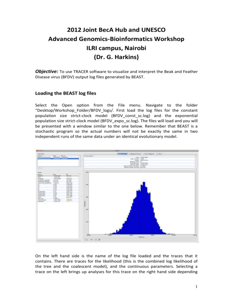
2012 Joint BecA Hub and UNESCO
Advanced Genomics-Bioinformatics Workshop
ILRI campus, Nairobi
(Dr. G. Harkins)
Objective: To use TRACER software to visualize and interpret the Beak and Feather
Disease virus (BFDV) output log files generated by BEAST.
Loading the BEAST log files
Select the Open option from the File menu. Navigate to the folder
“Desktop/Workshop_Folder/BFDV_logs/. First load the log files for the constant
population size strict-clock model (BFDV_const_sc.log) and the exponential
population size strict-clock model (BFDV_expo_sc.log). The files will load and you will
be presented with a window similar to the one below. Remember that BEAST is a
stochastic program so the actual numbers will not be exactly the same in two
independent runs of the same data under an identical evolutionary model.
On the left hand side is the name of the log file loaded and the traces that it
contains. There are traces for the likelihood (this is the combined log likelihood of
the tree and the coalescent model), and the continuous parameters. Selecting a
trace on the left brings up analyses for this trace on the right hand side depending
1
on tab that is selected. In the picture above, the log likelihood trace is selected for
the exponential strict-clock model and various statistics of these traces are shown
under the Estimates tab.
Note that the Effective Sample Sizes (ESS) values for all the traces are large (ESS
values less than 200 are highlighted in gold by Tracer). This is good. A high ESS value
means that the trace contained relatively few correlated samples and thus is a good
representation the posterior distribution. In the bottom right of the window is a
frequency plot of the samples, which as expected given the high ESS values, are
quite smooth.
We can improve these ESS values by setting the burn-in for the constant model at 5
million steps and the exponential model at 1 million steps.
Highlight both models and click on the tab labelled marginal density.
2
The statistics and their meaning are described below.
Mean
The mean value of the sampled trace across the chain (excluding the burnin).
Stdev
3
The standard deviation of the mean. This takes into account the effective
sample size so a small ESS will give a large Stdev.
Median
The median value of the sampled trace across the chain (excluding the burnin).
95% HPD Lower
The lower bound of the highest posterior density (HPD) interval. The HPD is a
credible set that contains 95% of the sampled values.
95% HPD Upper
The upper bound of the highest posterior density (HPD) interval. The HPD is a
credible set that contains 95% of the sampled values.
Auto-Correlation Time (ACT)
The number of states in the MCMC chain that two samples have to be from
each other for them to be uncorrelated. The ACT is estimated from the
samples in the trace (excluding the burn-in).
Effective Sample Size (ESS)
The ESS is the number of independent samples that the trace is equivalent to.
This is essentially the chain length (excluding the burn-in) divided by the ACT.
If we select the Trace we can view the raw trace, that is, the sampled values against
the step in the MCMC chain:
This is what we are aiming for - we call this plot the hairy caterpillar. There are no
obvious trends in the plot suggesting that the MCMC was still converging and there
are no large-scale fluctuations in the trace suggesting poor mixing.
4
As we are happy with the behaviour of log-likelihood, we can now move on to one of
the other parameters of interest: the mutation rate. Select siteModel.mu in the lefthand table. This is the mutation rate averaged over all three codon positions. Choose
the tab labelled Estimates to view a comparison of the estimates of the posterior
probability density of this parameter between models. You should see a graph
similar to this one showing the mean and the associated 95% HPD intervals for this
parameter.
View the density plot by selecting the tab labeled Marginal Density to see a plot of
these estimates.
5
As you can see the marginal posterior probability density is a reasonable looking
bell-shaped curve under both models. There is some stochastic noise that would be
reduced if we ran the chain for longer, but we already have a pretty good estimate
of the mean and credible interval for the mutation rate parameter under each
model.
6
Bayes Factor Testing
7
A value for the log10 Bayes factor > 3 indicates that one of the models has
significantly greater support that the other. In this case (BF = 1.47), therefore neither
8
model is a better fit to the data. i.e. under a strict-clock model we cannot
discriminate between a constant and exponentially growing population with this
data.
Given that we cannot discriminate between the different demographic models of
population size we can now focus on comparing across different clock models (strict
vs. relaxed). Close the exponential strict-clock log file and open the constant
population size relaxed-clock log file (BFDV_const_rc.log) located in the folder
labelled BFDV_logs.
Notice that unlike the constant population size strict clock model, the relaxed clock
ESS values for several of the traces are small (ESS values less than 200 and 100 are
highlighted in gold and red respectively by Tracer). This is not good. A low ESS value
means that the trace contained many correlated samples and thus is a not good
representation the posterior distribution. Comparing the traces for the log likelihood
parameter between the strict and relaxed-clock models explains why such low ESS
values were obtained.
9
Now compare the log likelihoods by clicking on the tab labelled Estimates
10
Bayes Factor Testing
In this case a BF of 194.962 indicates that the relaxed-clock nucleotide substitution is
a much better fit to the data than the strict-clock model assuming a constant
population size.
11
So far we have established that a) under a strict-clock model we cannot discriminate
between the constant and exponential demographic models and b) under a constant
population size model the relaxed-clock model provides a significantly better fit to
the data than the strict-clock model.
Finally we can compare whether either demographical model provides a better fit
under the relaxed-clock model. Close the constant strict clock log file and open the
exponential relaxed clock log file located in the folder xxx.
Notice that again the ESS values for many of the traces under the relaxed-clock
model are very small indeed. However, further examination of the trace file for
these parameters provides the cause of such low values. Examining the log likelihood
trace for the exponential growth model it becomes clear that the low ESS values are
caused by application of an inappropriately sized burn-in period.
12
If we correct for this by applying a burn-in value of 40 million steps to the
exponential relaxed-clock model the ESS values improve significantly but many
remain too small to represent the posterior distribution well. Essentially, this simply
looks as if we need to run the chain for longer. Given the lowest ESS (for the
coalescent likelihood) is 25.88, it would suggest that we have to run it for ~8 times
longer to get ESS values that are > 200.
13
If we ignore for the moment the small ESS values for these models and again
compare their fit to the data using Bayes factor testing we can see that a BF of 0.432
indicates that neither of the demographic models provides a better fit to the data
under a relaxed-clock model and therefore the results under both models should be
presented (Supplementary material).
In practice, we should rerun the Markov chain for much longer for all of the models
with ESS values of <200 for any of the traces and only then, compare using Bayes
factors or other tests.
14