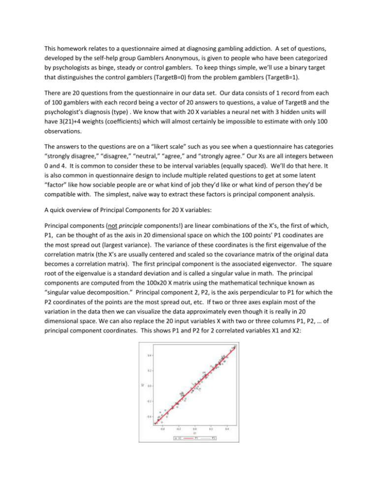
This homework relates to a questionnaire aimed at diagnosing gambling addiction. A set of questions,
developed by the self-help group Gamblers Anonymous, is given to people who have been categorized
by psychologists as binge, steady or control gamblers. To keep things simple, we’ll use a binary target
that distinguishes the control gamblers (TargetB=0) from the problem gamblers (TargetB=1).
There are 20 questions from the questionnaire in our data set. Our data consists of 1 record from each
of 100 gamblers with each record being a vector of 20 answers to questions, a value of TargetB and the
psychologist’s diagnosis (type) . We know that with 20 X variables a neural net with 3 hidden units will
have 3(21)+4 weights (coefficients) which will almost certainly be impossible to estimate with only 100
observations.
The answers to the questions are on a “likert scale” such as you see when a questionnaire has categories
“strongly disagree,” “disagree,” “neutral,” “agree,” and “strongly agree.” Our Xs are all integers between
0 and 4. It is common to consider these to be interval variables (equally spaced). We’ll do that here. It
is also common in questionnaire design to include multiple related questions to get at some latent
“factor” like how sociable people are or what kind of job they’d like or what kind of person they’d be
compatible with. The simplest, naïve way to extract these factors is principal component analysis.
A quick overview of Principal Components for 20 X variables:
Principal components (not principle components!) are linear combinations of the X’s, the first of which,
P1, can be thought of as the axis in 20 dimensional space on which the 100 points’ P1 coodinates are
the most spread out (largest variance). The variance of these coordinates is the first eigenvalue of the
correlation matrix (the X’s are usually centered and scaled so the covariance matrix of the original data
becomes a correlation matrix). The first principal component is the associated eigenvector. The square
root of the eigenvalue is a standard deviation and is called a singular value in math. The principal
components are computed from the 100x20 X matrix using the mathematical technique known as
“singular value decomposition.” Principal component 2, P2, is the axis perpendicular to P1 for which the
P2 coordinates of the points are the most spread out, etc. If two or three axes explain most of the
variation in the data then we can visualize the data approximately even though it is really in 20
dimensional space. We can also replace the 20 input variables X with two or three columns P1, P2, … of
principal component coordinates. This shows P1 and P2 for 2 correlated variables X1 and X2:
Homework Questions:
(1) Run the demo program Gamblers.sas being sure to fill in your AAEM library path in the first line.
Check to be sure the data got into your library.
The program creates 20 principal components Prin1 through Prin20. Look at the eigenvalues. They add
to n=20, the number of questions. Dividing the sum of the first k eigenvalues by 20 gives the proportion
of variation “explained by” the first k eigenvalues. What proportion _____ of the variation in all 20
questions is explained by the first three principal components?
The eigenvectors help us name the principal components. These are in fact the eigenvectors. To see
where I score on a principal component axis, I multiply each of my 20 answers by the associated
eigenvector entry (think of this as a weight) and add them up. That is, my row vector of answers is
multiplied by the column listed under PRIN1 to get my point’s first coordinate, by PRIN2 to get the
second, etc. My idea is to use the principal component scores (coordinates) to classify people. Look at
the questions with |weight|>0.3 in PRIN1. Do the same for PRIN2 and PRIN3. One analyst described
the questionnaire as looking at feelings, consequences, and excuses for gambling. From the weights,
match PRIN1 PRIN2 and PRIN3 with these three descriptors. For example, which one is the “feelings”
principal component axis?
(2) Using those three principal components, construct a neural network to identify the target variable
TargetB. That means we have rejected all of the original 20 questions and all but 3 of the principal
components. We did this outside EM but could have done it internally too. Set the variable Type to an
ID variable (why?). You can try this with default settings but that did not converge for me. How many
parameters would the default settings attempt to estimate if you use all three principal componets?
_____ To reduce the number of parameters even further than the principal components do, go to the
network architecture ellipsis in the properties panel and set the number of hidden units to 2 rather than
3. Don’t forget to declare the response target to be binary and let the other numeric variables be
interval. What is the range ___ to ___ of prin3? Set prin3 to 0. Make a 3D graph of Z = the probability
of being a problem gambler = P_TargetB1 versus the prin1 and prin2 (X, Y) coordinates. You can do
this by copying the neural net code and inserting it in a grid-producing loop like that in the demo
Neural3_Framingham.sas. It should look something like this, a somewhat interesting wrinkled surface.
Probability surface at excuses = 0
Predicted: TargetB=1
1.00
0.67
0.33
4.50
1.17
Consequences
0.00
4.50
-2.17
1.17
Feelings
-2.17
-5.50
-5.50
Just use the default labels rather than relabelling the axes as done above.
Optionally you might want to investigate the effect of different prin3 settings on this graph.
Notes: (no answer required).
Note 1: to use your model, you would ask a person to fill in the questionnaire. You would take their 20
answers and compute their location (scores) in the three dimensional (prin1, prin2, prin3) space then
get the predicted probability of being a problem gambler (i.e. not control) from the Neural Net model.
Note 2: Under the modify subtab there is a principal components node that you can use within
enterprise miner. In that way EM will calculate the principal component scores for scoring data set that
you submit.
Note 3: A more sophisticated axis computation than principal components is given by a technique called
factor analysis (PROC FACTOR) which is similar to, but not the same as, principal components.
Note 4: 100 observations is not anywhere near a large data set, likely not a strong enough set of data to
support a somewhat complex nonlinear model like a neural net. This is likely why we had to reduce the
number of hidden units.