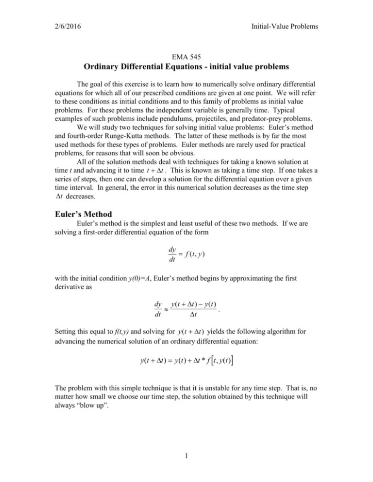
2/6/2016
Initial-Value Problems
EMA 545
Ordinary Differential Equations - initial value problems
The goal of this exercise is to learn how to numerically solve ordinary differential
equations for which all of our prescribed conditions are given at one point. We will refer
to these conditions as initial conditions and to this family of problems as initial value
problems. For these problems the independent variable is generally time. Typical
examples of such problems include pendulums, projectiles, and predator-prey problems.
We will study two techniques for solving initial value problems: Euler’s method
and fourth-order Runge-Kutta methods. The latter of these methods is by far the most
used methods for these types of problems. Euler methods are rarely used for practical
problems, for reasons that will soon be obvious.
All of the solution methods deal with techniques for taking a known solution at
time t and advancing it to time t  t . This is known as taking a time step. If one takes a
series of steps, then one can develop a solution for the differential equation over a given
time interval. In general, the error in this numerical solution decreases as the time step
t decreases.
Euler’s Method
Euler’s method is the simplest and least useful of these two methods. If we are
solving a first-order differential equation of the form
dy
 f (t, y )
dt
with the initial condition y(0)=A, Euler’s method begins by approximating the first
derivative as
dy y (t  t )  y (t )

.
dt
t
Setting this equal to f(t,y) and solving for y (t  t ) yields the following algorithm for
advancing the numerical solution of an ordinary differential equation:
y(t  t )  y(t )  t * f t , y(t )
The problem with this simple technique is that it is unstable for any time step. That is, no
matter how small we choose our time step, the solution obtained by this technique will
always “blow up”.
1
2/6/2016
Initial-Value Problems
The Fourth-Order Runge-Kutta Method
The fourth-order Runge-Kutta algorithm is:
k1  t * f ( t , y ( t ))
k
t
, y( t )  1 )
2
2
k
t
k3  t * f ( t  , y ( t )  2 )
2
2
k 4  t * f ( t  t , y ( t )  k3 )
k  2( k 2  k3 )  k 4
y ( t  t )  y ( t )  1
6
k 2  t * f ( t 
As before, a series of these steps can be used to generate a full numerical solution to an
initial value problem. This method is very powerful and is widely used.
The Solution of Second Order Equations
Our next task is to solve a second-order ordinary differential equation. The
Runge-Kutta technique is designed to solve systems of first order equations, so we must
first convert our second-order equation into two first order equations. For example,
suppose we have the equation and initial conditions
d2y
dy
 c  ky  F sin( t )
2
dt
dt
y (0)  1
dy
(0)  0
dt
m
We can define the intermediate variable z(t) as
dy
 z  g (t , y, z )
dt
which gives us:
dy
z
dt
dz  c z  k y  F sin( t )

dt
m
y ( 0)  1
z ( 0)  0
2
2/6/2016
Initial-Value Problems
This gives us two first order equations. We can now solve these using Runge-Kutta.
Runge-Kutta for Two, Coupled First-Order Equations
To solve a system of two, coupled equations, we modify the earlier Runge-Kutta
algorithm according to:
k1  t * g (t , y (t ), z (t ))
l1  t * f (t , y (t ), z (t ))
t
k
l
k 2  t * g ( t  , y ( t )  1 , z ( t )  1 )
2
2
2
t
k1
l1
l2  t * f (t  , y ( t )  , z (t )  )
2
2
2
t
k
l
k 3  t * g ( t  , y ( t )  2 , z ( t )  2 )
2
2
2
t
k
l
l3  t * f (t  , y (t )  2 , z (t )  2 )
2
2
2
k 4  t * g (t  t , y (t )  k 3 , z (t )  l3 )
l4  t * f (t  t , y (t )  k 3 , z (t )  l3 )
k1  2 * ( k 2  k 3 )  k 4
6
l  2 * ( l2  l3 )  l4
z (t  t )  z (t )  1
6
y (t  t )  y (t ) 
This can be used to solve nearly any second-order initial value problem.
The Excel macro to carry this out looks like:
Function g(t, y, z)
g = z
End Function
Function f(t, y, z)
mass = 1
omega = 2
c = 1
k = 3
fo = 4
f = (fo * Sin(omega * t) - k * y - c * z) / mass
End Function
3
2/6/2016
Initial-Value Problems
Sub domanyrungthree()
Dim writeinterval As Integer
[A13:B1015].Clear
ynot = Cells(4, 2).Value
znot = Cells(5, 2).Value
EndTime = Cells(6, 2).Value
Steps = Cells(7, 2).Value
StartTime = 0
t = StartTime
h = (EndTime - StartTime) / Steps
y = ynot
z = znot
Cells(12, 1).Select
Application.ScreenUpdating = False
ActiveCell.Value = "Time"
ActiveCell.Offset(0, 1).Value = "Position"
ActiveCell.Offset(1, 0).Value = t
ActiveCell.Offset(1, 1).Value = y
ActiveCell.Offset(1, 0).Select
writeinterval = 5 '
For i = 1 To Steps
Call runge(h, t, y, z, ynew, znew)
t = t + h
y = ynew
z = znew
ActiveCell.Offset(1, 0).Value = t
ActiveCell.Offset(1, 1).Value = y
ActiveCell.Offset(1, 0).Select
Next
Cells(1, 1).Select
Application.ScreenUpdating = True
End Sub
Sub runge(h,
k1 = h *
l1 = h *
k2 = h *
l2 = h *
k3 = h *
l3 = h *
k4 = h *
l4 = h *
ynew = y
znew = z
End Sub
t, y, z, ynew, znew)
g(t, y, z)
f(t, y, z)
g(t + 0.5 * h, y + 0.5 * k1, z +
f(t + 0.5 * h, y + 0.5 * k1, z +
g(t + 0.5 * h, y + 0.5 * k2, z +
f(t + 0.5 * h, y + 0.5 * k2, z +
g(t + h, y + k3, z + l3)
f(t + h, y + k3, z + l3)
+ (k1 + 2 * (k2 + k3) + k4) / 6
+ (l1 + 2 * (l2 + l3) + l4) / 6
4
0.5
0.5
0.5
0.5
*
*
*
*
l1)
l1)
l2)
l2)