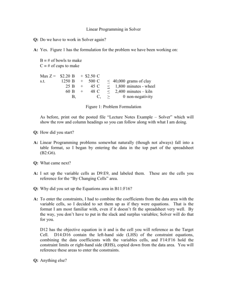
Linear Programming in Solver
Q: Do we have to work in Solver again?
A: Yes. Figure 1 has the formulation for the problem we have been working on:
B  # of bowls to make
C  # of cups to make
Max Z = $2.20 B
s.t.
1250 B
25 B
60 B
B,
+ $2.50 C
+ 500 C
+
45 C
+
48 C
C,
< 40,000 grams of clay
< 1,800 minutes - wheel
< 2,400 minutes – kiln
>
0 non-negativity
Figure 1: Problem Formulation
As before, print out the posted file “Lecture Notes Example – Solver” which will
show the row and column headings so you can follow along with what I am doing.
Q: How did you start?
A: Linear Programming problems somewhat naturally (though not always) fall into a
table format, so I began by entering the data in the top part of the spreadsheet
(B2:G6).
Q: What came next?
A: I set up the variable cells as D9:E9, and labeled them. These are the cells you
reference for the “By Changing Cells” area.
Q: Why did you set up the Equations area in B11:F16?
A: To enter the constraints, I had to combine the coefficients from the data area with the
variable cells, so I decided to set them up as if they were equations. That is the
format I am most familiar with, even if it doesn’t fit the spreadsheet very well. By
the way, you don’t have to put in the slack and surplus variables; Solver will do that
for you.
D12 has the objective equation in it and is the cell you will reference as the Target
Cell. D14:D16 contain the left-hand side (LHS) of the constraint equations,
combining the data coefficients with the variables cells, and F14:F16 hold the
constraint limits or right-hand side (RHS), copied down from the data area. You will
reference these areas to enter the constraints.
Q: Anything else?
A: I am assuming you remember how to use the Solver dialogue box to enter all the
information. I have learned that if you ask Solver to be too precise (Precision and
Convergence in the “Options” box), then it gets sulky and declares “The conditions
for Assume Linear Model are not satisfied.” That is ridiculous, but that is what it
does. How you set up the constraints determines how precise you can be (which
makes even less sense). It seems to fall apart somewhere between 15 and 20 decimal
places.
This is important because if you get that error message it will give you the solution on
the spreadsheet, but will not give you the “Answer” and “Sensitivity Analysis”
reports and you need the sensitivity analysis report.
Q: Assuming we have gotten Solver to run, how do we read the “Answer” and
“Sensitivity Analysis” reports?
A: First, after you get the message “Solver found a solution,” on right-hand side of the
box is a list labeled “Reports,” and in that list are three options: Answer, Sensitivity
and Limits. The “Limits” report is not relevant to LP (well, it is, a little, but we won’t
use it). The only thing you need the “Answer” report for is the values of the Slack
variables, and you could calculate those on your spreadsheet if you wanted to. The
“Sensitivity” report, though, is useful. It gives you several pieces of information,
such as allowable variation for the objective and constraint limit coefficients (shown
as “Allowable Increase” and “Allowable Decrease,” and the shadow prices (also
known as dual values or reduced costs) for the variables (decision and slack).
Q: How do we use the allowable variation?
A: You can use it as we did for a payoff table, and compare it to the amount of variation
you expect, or you can use them to check specific changes to individual coefficients.
Q: Could you show us some examples of checking specific changes?
A: I’ll begin by copying the sensitivity analysis tables to these notes:
Coeff
Bowls
Cups
2.2
2.5
Allowable
Increase
0.925
1.460
Allowable
Decrease
0.811
0.740
Clay
Wheel
Kiln
Constr
RHS
40,000
1,800
2,400
Allowable
Increase
1E+30
450
205.7
Allowable
Decrease
6,000
300
480
The allowable increase and decrease are the amounts the coefficients can change by
not change to. These are the ranges where your current solution would still be
acceptable to you (it will change in minor respects, not in any major respect). By the
way, “1E+30” is Solver’s way of saying “infinity.” That means that any increase is
allowable. Any decrease being allowable would have a limit of “1E-30.”
Now I have some questions for you.
Q: If the profit on bowls decreases by $0.50, would you still use the same solution?
A: Yes, because $0.50 < $0.811, the allowable decrease.
Q: If the profit on cups increases to $4.00 per cup, would you still use the same solution?
A: No, because $4.00 is not < $3.96 (the coefficient plus the allowable increase).
Q: If the amount of clay available decreases by 10 kg, would you still use the same
solution?
A: No, because -10,000 g is less than -6,000 g, the allowable decrease.
Q: Do you get the idea?
A: Yes, it is pretty simple.
Q: In that case, if the wheel and the kiln are both out of order for 200 minutes, would
you still use the same solution?
A: Well, 200 < 300 for the wheel and 200 < 480 for the kiln, so, yes.
D: Wrong.
Q: Would the answer be “No,” because there are two changes?
A: Wrong.
Q: What is the answer?
A: I don’t know.
Q: Are you saying you don’t know, or that the answer is “I don’t know?”
A: The answer is “I don’t know”
Q: Why is that the answer?
A: You were close when you asked if it was because I made two changes at once. If you
remember, when we did sensitivity analysis for the payoff table, I always made sure I
changed only one number at a time. The ranges in the LP sensitivity analysis are
based on the same idea – one coefficient changing at a time. If two coefficients
change, the ranges no longer apply. The current solution might be good, or it might
not. We simply don’t know.
Q: What do we do?
A: Enter both the changed coefficients into the spreadsheet and re-solve the problem.
Q: So, let’s try that again: if the profit on cups decreases by $0.50 and the amount of clay
available doubles, would you still use the current solution?
A: I don’t know.
D: Wrong.
Q: What?
A: Sorry, but you are wrong. There are two tables in the sensitivity analysis and they are
calculated independently of one another. That means one number can change in one
table and one number can change in the other table, and we treat the changes just like
any other –we see if the changes are within the allowable changes.
Q: So, is the current solution still good?
A: Well, for cups, $0.50 < $0.74, so that one is OK, and the allowable increase for clay
is infinity, so doubling would be no problem, so, yes.
Q: How can an allowable increase be infinity?
A: If you look at the answer report, or the graph for the problem, or calculate it yourself,
you will find out that there are 6,000 g of clay left unused at the optimal solution. If
you failed to use all the clay that is currently available, having more clay would only
increase that unused amount, not change the solution.
Q: Are there any more tricks to sensitivity analysis?
A: Not for the allowable increases and decreases, but we do need to talk about shadow
prices.
Q: What are shadow prices?
A: Another name for reduced costs, which we talked about (a lot) when learning how the
LP algorithm works. You may remember that the reduced cost tells you the effect on
the objective for a 1-unit change in a variable’s value. Well, that still holds true, but
now we can use that information to decide whether or not to re-supply, or for this
problem, whether or not to work overtime.
The Sensitivity report tells us the shadow prices are $0.0/g for clay, $0.03/minute for
time on the wheel, and $0.025/minute for the kiln. We’re not interested in getting
more clay; we already have some left over. However, converting the shadow prices
to hourly rates, that $1.80 extra profit for an extra hour on the wheel and $1.50 extra
profit for an extra hour in the kiln.
Q: How do we use that information?
A: By comparing it to another number. Suppose you know that running the kiln for an
extra hour will cause a small part to break. Replacing the part costs $2.00, so the
increased profit (the shadow price of $1.50 per hour) is less than the increase in cost
of $2.00, so we’re not interested.
Q: Is there anything else we need to know about reading the Solver output?
A: Not really. Larger problems seem more complex, because they have more data, but it
is really only the same information, over and over. So, take it in small pieces,
understand each part, and you should be OK.