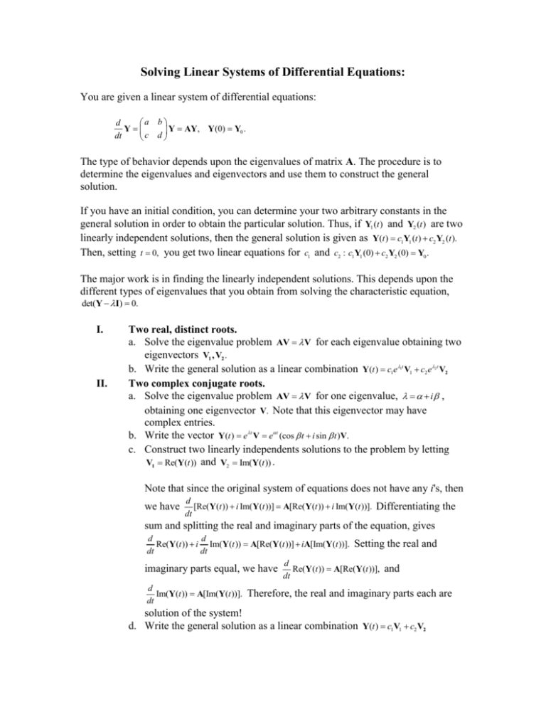
Solving Linear Systems of Differential Equations:
You are given a linear system of differential equations:
a b
d
Y
 Y  AY, Y(0)  Y0 .
dt
c d
The type of behavior depends upon the eigenvalues of matrix A. The procedure is to
determine the eigenvalues and eigenvectors and use them to construct the general
solution.
If you have an initial condition, you can determine your two arbitrary constants in the
general solution in order to obtain the particular solution. Thus, if Y1 (t ) and Y2 (t ) are two
linearly independent solutions, then the general solution is given as Y(t )  c1Y1 (t )  c2 Y2 (t ).
Then, setting t  0, you get two linear equations for c1 and c2 : c1Y1 (0)  c2 Y2 (0)  Y0 .
The major work is in finding the linearly independent solutions. This depends upon the
different types of eigenvalues that you obtain from solving the characteristic equation,
det(Y  I)  0.
I.
Two real, distinct roots.
a. Solve the eigenvalue problem AV   V for each eigenvalue obtaining two
eigenvectors V1 , V2 .
b. Write the general solution as a linear combination Y(t )  c1e t V1  c2 e t V2
Two complex conjugate roots.
a. Solve the eigenvalue problem AV   V for one eigenvalue,     i ,
obtaining one eigenvector V. Note that this eigenvector may have
complex entries.
b. Write the vector Y(t )  et V  e t (cos  t  i sin  t )V.
c. Construct two linearly independents solutions to the problem by letting
V1  Re(Y(t )) and V2  Im(Y(t )) .
1
II.
2
Note that since the original system of equations does not have any i's, then
we have
d
[Re(Y(t ))  i Im(Y(t ))]  A[Re(Y(t ))  i Im(Y(t ))].
dt
Differentiating the
sum and splitting the real and imaginary parts of the equation, gives
d
d
Re(Y(t ))  i Im(Y(t ))  A[Re(Y(t ))]  iA[Im(Y(t ))]. Setting the real and
dt
dt
d
imaginary parts equal, we have Re(Y(t ))  A[Re(Y(t ))], and
dt
d
Im(Y(t ))  A[Im( Y(t ))]. Therefore, the real and imaginary parts each are
dt
solution of the system!
d. Write the general solution as a linear combination Y(t )  c1V1  c2 V2
III.
IV.
One Repeated Root
a. Solve the eigenvalue problem AV   V for the one eigenvalue obtaining
the first eigenvector V1 .
b. Solve the eigenvalue problem AV2   V2  V1 for V2 .
c. The general solution is then given by Y(t )  c1et V1  c2 et (V2  tV1 ) .
Examples
 4 2
.
 3 3
a. A  
0
4
2
3
3
Eigenvalues: 0  (4   )(3   )  6
Thus,   1, 6.
0    7  6
0  (  1)(  6)
2
Eigenvectors:
  1:
  6:
 4 2   v1   v1 

    
 3 3   v2   v2 
 3 2   v1   0 

    
 3 2   v2   0 
 v1 
 4 2   v1 

   6 
 3 3   v2 
 v2 
 2 2   v1   0 

    
 3 3   v2   0 
v   2 
 v   1
3v1  2v2  0,   1     . 2v1  2v2  0,   1     .
 v2   3 
 v2   1
Y(t )  c1e1t V1  c2 e2t V2
2
6 t  1
  c2 e  
 3 
 1
General Solution: Y(t )  c1et 
 2c et  c e6t 
  1 t 2 6t  .
 3c1e  c2 e 
 3 5 
b. A  
.
 1 1 
0
Eigenvalues:
3
1
5
1  
0  (3   )( 1   )  6
0   2  2  2

(2)  4  4(1)(2)
 1  i.
2
Thus,   1  i,1  i.
Eigenvectors:
  1 i :
 v1 
 3 5   v1 

    (1  i )  
 1 1   v2 
 v2 
5   v1   0 
2i

    
2  i   v2   0 
 1
 v  2i
(2  i )v1  5v2  0,   1   
.
 v2   1 
Complex Solution:
2i
(1 i ) t  2  i 
et 
e


1


 1 
2i
 et (cos t  i sin t ) 

 1 
 (2  i )(cos t  i sin t ) 
 et 

cos t  i sin t


 (2 cos t  sin t )  i (cos t  2sin t ) 
 et 

cos t  i sin t


2
cos
t

sin
t
cos
t

2sin
t



t
 et 
  ie 
.
cos t
sin t




General Solution:
 2 cos t  sin t 
t  cos t  2sin t 
Y(t )  c1et 
  c2 e 

cos
t
sin t




c
(2
cos
t

sin
t
)

c
(cos
t

2sin
t
)


2
 et  1
.
c
cos
t

c
sin
t

1
2

 2c1  c2  t
 2c2  c1 
  e sin t 
.
 c1 
 c2 
Note: This can be rewritten as Y(t )  et cos t 
 7 1
.
9 1 
c. A  
0
7
1
9
1 
0  (7   )(1   )  9
Eigenvalues: 0   2  8  16
0  (  4)
.
2
Thus,   4.
Eigenvectors:
  4:
 v1 
 7 1  v1 

   4 
 9 1   v2 
 v2 
 3 1   v1   0 

    
 9 3   v2   0 
 v  1
3v1  v2  0,   1     .
 v2   3 
Second Linearly Independent Solution:
Solve AV2   V2  V1
 7 1  u1   u1   1 

   4    
 9 1   u2   u2   3 
 3 1   u1   1 

    
 9 3   u2   3 
3u1  u2  1 
 u1   1 
      .
9u1  3u2  3
 u2   2 
General Solution:
Y (t )  c1et V1  c2 e  t (V2  tV1 )
 1   1  
1
Y (t )  c1e 4t    c2 e 4t    t   
 3
 2   3  
 c  c (1  t ) 
 e 4t  1 2
.
 3c1  c2 (2  3t ) 