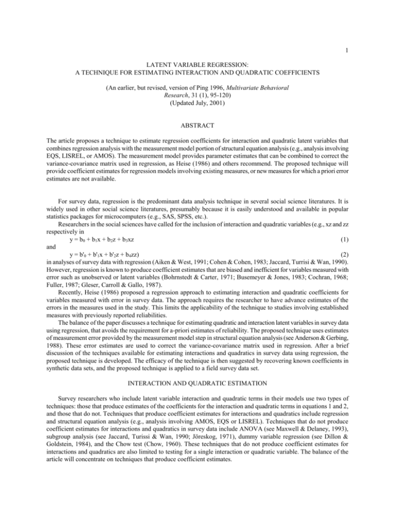
1
LATENT VARIABLE REGRESSION:
A TECHNIQUE FOR ESTIMATING INTERACTION AND QUADRATIC COEFFICIENTS
(An earlier, but revised, version of Ping 1996, Multivariate Behavioral
Research, 31 (1), 95-120)
(Updated July, 2001)
ABSTRACT
The article proposes a technique to estimate regression coefficients for interaction and quadratic latent variables that
combines regression analysis with the measurement model portion of structural equation analysis (e.g., analysis involving
EQS, LISREL, or AMOS). The measurement model provides parameter estimates that can be combined to correct the
variance-covariance matrix used in regression, as Heise (1986) and others recommend. The proposed technique will
provide coefficient estimates for regression models involving existing measures, or new measures for which a priori error
estimates are not available.
For survey data, regression is the predominant data analysis technique in several social science literatures. It is
widely used in other social science literatures, presumably because it is easily understood and available in popular
statistics packages for microcomputers (e.g., SAS, SPSS, etc.).
Researchers in the social sciences have called for the inclusion of interaction and quadratic variables (e.g., xz and zz
respectively in
y = b0 + b1x + b2z + b3xz
(1)
and
y = b'0 + b'1x + b'2z + b4zz)
(2)
in analyses of survey data with regression (Aiken & West, 1991; Cohen & Cohen, 1983; Jaccard, Turrisi & Wan, 1990).
However, regression is known to produce coefficient estimates that are biased and inefficient for variables measured with
error such as unobserved or latent variables (Bohrnstedt & Carter, 1971; Busemeyer & Jones, 1983; Cochran, 1968;
Fuller, 1987; Gleser, Carroll & Gallo, 1987).
Recently, Heise (1986) proposed a regression approach to estimating interaction and quadratic coefficients for
variables measured with error in survey data. The approach requires the researcher to have advance estimates of the
errors in the measures used in the study. This limits the applicability of the technique to studies involving established
measures with previously reported reliabilities.
The balance of the paper discusses a technique for estimating quadratic and interaction latent variables in survey data
using regression, that avoids the requirement for a-priori estimates of reliability. The proposed technique uses estimates
of measurement error provided by the measurement model step in structural equation analysis (see Anderson & Gerbing,
1988). These error estimates are used to correct the variance-covariance matrix used in regression. After a brief
discussion of the techniques available for estimating interactions and quadratics in survey data using regression, the
proposed technique is developed. The efficacy of the technique is then suggested by recovering known coefficients in
synthetic data sets, and the proposed technique is applied to a field survey data set.
INTERACTION AND QUADRATIC ESTIMATION
Survey researchers who include latent variable interaction and quadratic terms in their models use two types of
techniques: those that produce estimates of the coefficients for the interaction and quadratic terms in equations 1 and 2,
and those that do not. Techniques that produce coefficient estimates for interactions and quadratics include regression
and structural equation analysis (e.g., analysis involving AMOS, EQS or LISREL). Techniques that do not produce
coefficient estimates for interactions and quadratics in survey data include ANOVA (see Maxwell & Delaney, 1993),
subgroup analysis (see Jaccard, Turissi & Wan, 1990; Jöreskog, 1971), dummy variable regression (see Dillon &
Goldstein, 1984), and the Chow test (Chow, 1960). These techniques that do not produce coefficient estimates for
interactions and quadratics are also limited to testing for a single interaction or quadratic variable. The balance of the
article will concentrate on techniques that produce coefficient estimates.
2
STRUCTURAL EQUATION TECHNIQUES
Kenny and Judd (1984), among others (e.g., Bollen 1995, Hayduk, 1987; Jaccrd & Wan 1995; Jöreskog & Yang
1996; Ping 1995, 1996; Wong & Long, 1987), have proposed an approach to specifying interaction and quadratic latent
variables using structural equation analysis. In structural equation analysis the measured variables (indicators) are
assumed to be linear functions of their unobserved (latent) variable. For an indicator x this relationship is specified as
Var(x) = λX2Var(ξX) + Var(εX) ,
(3)
where Var(a) is the variance of a, λX is the (factor) loading of x on the latent variable ξX, εX is the error in measuring x,
and ξX and εX are independent (Jöreskog, 1973; Keesling, 1972; Wiley, 1973). The Kenny and Judd approach involves
specifying the indicators of a latent variable interaction, ξXZ for example, by using all possible products of the indicators
of the latent variables ξX and ξZ. In particular for ξX and ξZ with indicators x1, x2, z1, and z2, respectively, ξXZ would have
the indicators x1z1, x1z2, x2z1, and x2z2.1 Under certain conditions the variance of these indicator products is given by
Var(xizj) = Var((λXiξX + εXi)(λZjξZ + εZj))
= λXiλZjVar(ξXZ) + λXiVar(ξX)εZj + λZjVar(ξZ)εXi + Var(εXi)Var(εZj) .
(4)
Specification of these indicator products is tedious however. The Kenny and Judd approach requires the specification
of four dummy (non-linear) variables, one for λXiλZj, and one for each of the last three terms of equation 4. Hence a total
of sixteen dummy variables would be required for the four product indicators of ξXZ. For models with several interactions
or quadratics, or several indicators per variable, these dummy variables can overwhelm the model. For example a model
with two linear latent variables (e.g., ξX and ξZ) having six indicators each, one interaction, and two quadratic variables
requires the specification of three hundred and seventy-two additional dummy variables.2 Aiken and West (1991) noted
that this approach has been difficult for researchers to implement.
Regression Techniques
Perhaps for these reasons regression continues to be a popular alternative to structural equation analysis for
estimating interactions and quadratic effects among latent variables. Two regression approaches are available.
Researchers can ignore measurement error, sum the items to form a single measure of each concept, and form arithmetic
products of these summed measures to create interaction and quadratic variables. For example, the interaction variable
corresponding to the summed variables X = x1 + x2 and Z = z1 + z2 would have the form XZ = (x1 + x2)(z1 + z2).
Quadratic variables would be similarly constructed. These variables can then be added to the regression model. However,
this approach has been criticized for its biased and inefficient coefficient estimates for both the summed variables and the
interactions and quadratics (Bohrnstedt & Carter, 1971; Busemeyer & Jones, 1983; Cochran, 1968; Fuller, 1987; Gleser,
Carroll & Gallo, 1987).
Warren, White and Fuller (1974) and Heise (1986) proposed an alternative approach for regression and variables
measured with error, that involved correcting the regression moment matrix using appropriate error variance terms.
Consider the variable x given by x = XT + ex , where x is the observed score, XT is the true score, and ex is error. The
variance of the true score XT could be estimated using the variance of the observed score x and the variance of the error
ex, and the regression variance-covariance matrix could be corrected for this error. Specifically,
Var(x) = Var(XT) + Var(ex)
(5)
where XT and ex are assumed to be uncorrelated. Hence
Var(ex) = Var(x) - Var(XT)
= Var(x) - ρXXVar(X)
= Var(x)(1 - ρXX)
where
ρXX = Var(XT)/Var(x) = the (a-priori) reliability of x.
For an interaction variable xz,
Var(XTZT) = Var[(x-ex)(z-ez)]
= Var(xz - xez - zex + exez)
= Var(xz) - Var(z)Var(ex) - Var(x)Var(ez)+ Var(ex)Var(ez)
= Var(xz) - Var(z)Var(x)(1 - ρXX) - Var(x)Var(z)(1 - ρZZ)
+ Var(x)(1 - ρXX)Var(z)(1 - ρZZ)
(see Bohrnstedt & Goldberger, 1969) could replace Var(xz) in the regression variance-covariance matrix, assuming x and
3
z have a multivariate normal distribution with zero mean.
While useful, this approach is limited to situations where the a-priori errors or reliabilities of x and z are known.
Nevertheless, a similar correction approach could be taken using a structural equation analysis. This approach is
developed next.
A PROPOSED ESTIMATION TECHNIQUE
Structural equation modeling packages such as AMOS, EQS and LISREL can provide a straightforward estimate of
λX, Var(ξX), and Var(εX) in equation 3 using the so-called measurement model (see Anderson & Gerbing, 1982; 1988)
(see also Byrne, 1989). This measurement model is intended to gauge the adequacy of the assignment of indicators to
latent variables, and in the process it produces estimates of the parameters in equation 3 (i.e., Var(ε X), λX and Var(ξX)).
For variables formed as sums of indicators such as X = x1 + x2 , equation 3 becomes
Var(X) = Var(x1 + x2)
= Var[(λX1ξX + εX1) + (λX2ξX + εX2)]
= Var((λX1 + λX2)ξX) + Var(εX1) + Var(εX2)
= Var(ΛXξX) + θX,
= ΛX2Var(ξX) + θX,
(6)
where ΛX = λX1 + λX2, θX = Var(εX1) + Var(εX2), x1 and x2 are independent of εX1 and εX2, εX1 and εX2 are independent of
each other, and x1 and x2 are multivariate normal with zero means. Since estimates of ΛX = λX1 + λX2, θX = Var(εX1) +
Var(εX2), and Var(ξX) are available in a measurement model for ξX, they can be used to correct Var(X), and provide a
consistent estimate of Var(ξX). Rearranging equation 6, Var(X) in a regression variance-covariance matrix could be
replaced by an estimate of Var(ξX)
Var(ξX) = (Var(X) - θX)/ΛX2 .
(7)
CORRECTION EQUATIONS
The balance of the regression variance-covariance matrix could be corrected in a similar manner, using combinations
of the uncorrected variance-covariance matrix entries and measurement model estimates. For example, consider the
following regression model,
Y = b0 + b1X + b2Z + b3V + b4W + b5XX + b6ZZ + b7XZ + b8VW + b9VZ ,
(8)
where X, Z, V, W and Y are sums of indicators and of the form
Q = q1 + q2 ,
XX, ZZ, XZ, VW, and VZ are of the form
PQ = (p1+p2)(q1+q2) ,
and p1, p2, q1 and q2 are indicators meeting the equation 6 conditions.
The correction for the diagonal term Var(X) in the variance-covariance matrix for equation 8 is given by equation 7
and the corrections for Var(Z), Var(V), Var(W), and Var(Y) are similar to those shown in equation 7. Under the
assumptions for equation 6, the corrections for the other terms in the variance-covariance matrix for equation 8 can be
determined. For example, the corrections for the equation 8 variance-covariance matrix diagonal terms composed of
interactions such as Var(XZ), Var(VW) and Var(VZ) are given by
Var(ξXξZ) = (Var(XZ) - Var(ξX)ΛX2θZ - Var(ξZ)ΛZ2θX -θXθZ)/ΛX2ΛZ2
(9)
where ΛX = λx1 + λx2, ΛZ = λz1 + λz2, θX = Var(εx1) + Var(εx2), and θZ = Var(εz1) + Var(εz2) (see Appendix A).
The correction for quadratics such as Var(XX) and Var(ZZ) is similar
Var(ξXξX) = (Var(XX) - 4Var(ξX)ΛX2θX - 2θX2)/ΛX4 .
(10)
Off diagonal terms composed of linear variables such as Cov(X,Z), are given by
Cov(ξX,ξZ) = Cov(X,Z)/ΛXΛZ .
(11)
Other combinations of linear terms such as Cov(X,Y), Cov(X,V), Cov(X,W), Cov(Z,Y), Cov(Z,V), Cov(Z,W) and
Cov(V,W) are similar.
Mixed off-diagonal terms composed of linear and interaction or quadratic variables are also corrected. For example,
terms such as Cov(V,XZ) are corrected as follows
Cov(ξV,ξXξZ) = Cov(V,XZ)/ΛVΛXΛZ .
(12)
The other combinations of linear and interaction or quadratic terms such as Cov(X,XX), Cov(Z,XZ), etc. are similar.
For the correction of off diagonal combinations of interactions and quadratics there are several cases: a covariance
term composed of two quadratics, two interactions, or an interaction and a quadratic. The covariance of a quadratic and
4
an interaction with a common linear term such as Cov(XX,XZ) is corrected with
Cov(ξXξX,ξXξZ) = (Cov(XX,XZ) - 2Cov(ξX,ξZ)ΛXΛZθX)/ΛX3ΛZ .
(13)
Other combinations of interactions or quadratics are corrected similarly. For example, a covariance with two interactions
with a common linear term such as Cov(VW,VZ) is corrected with
Cov(ξVξW,ξVξZ) = (Cov(VW,VZ) - Cov(ξW,ξZ)ΛWΛZθV)/ΛV2ΛWΛZ .
(14)
A covariance with a combination of interactions or quadratics with no common terms such as Cov(XZ,VW) or
Cov(XX,ZZ) is corrected with
Cov(ξXξZ,ξVξW) = Cov(XZ,VW)/ΛXΛZΛVΛW .
(15)
Equations 7 and 9-15 generalize to an arbitrary number of indicators for X, Z, V, W and Y (see Appendix A).
SYNTHETIC DATA EXAMPLES
To gauge the efficacy of this technique it was used to recover known coefficients in synthetic data sets. Using a
normal random number generator, data sets composed of 100 replications of samples of 50, 100, and 150 cases were
created. Each replication was generated using the Table 1 population characteristics for x1, x2, z1, z2, t1, t2 and y in the
equation
Y = βY,XX + βY,ZZ + βY,TT + βY,XZXZ + βY,XXXX + ζY
(16)
(see Appendix B for details).To gauge the effects of varying the simulation conditions the process was repeated for two
additional levels of latent variable reliability (see Table 1).
The equation 16 model was estimated for each replication by creating the variables X (= [x1+x2]/2), Z (= [z1+z2]/2),
T (= [t1+t2]/2), XX (= X*X), XZ (= X*Z), and Y (= y, a single indicator) in each case. 3 Then the linear-terms-only
measurement model associated with equation 16 (i.e., involving only X, Z, T and Y-- see Figure 1) was estimated using
EQS and maximum likelihood estimates. Specifically the λ's, θε's and the variances and covariances of the latent variables
ξX, ξZ, ξT, and ξY were estimated. This produced estimates of the λ's, θε's and Var(ξ)'s for use in equations 7 and 9-13.
After using equation 7 and 9-13 to correct the equation 16 variance-covariance matrix, the coefficients in equation 16
were estimated using this corrected matrix and ordinary least squares regression. The results are shown in Table 2.
To obtain a basis for comparison uncorrected regression estimates were also generated for each replication. These
estimates used the uncorrected equation 16 variance-covariance matrix and ordinary least squares. The results are also
shown in Table 2, and will be discussed later.
To illustrate the use of the proposed technique a field survey data analysis involving interaction and quadratic latent
variables is presented.
A FIELD SURVEY EXAMPLE
As part of a study of reactions to changes in overall inter-group satisfaction with an exchange relationship (e.g., a
firm selling to another firm) data were gathered using multiple Likert items measuring overall satisfaction (SAT) of the
subject group with the partner group, the attractiveness of the best alternative group (ALT), and the opportunism (OPP)
(self interest seeking with guile, Williamson, 1975) (which can plausibly be viewed as a form of instrumental aggression)
committed by the subject group on the partner group (see Ping, 1993).
Since the purpose is to illustrate the use of the proposed estimation technique the study will simply be summarized.
SAT was measured using a seven-item scale, ALT used six items, and OPP was measured with eight items. The
anticipated relationships among the study concepts were
OPP = b1SAT + b2ALT + ζ.
(17)
Opportunism was expected to be negatively associated with satisfaction and positively associated with the attractiveness
of the best alternative.
Because alternative attractiveness was a new measure developed for this study, an a-priori estimate of its reliability
was not available, and the approaches suggested by Heise (1986) or Feucht (1989) were not feasible. In addition, a
structural equation analysis using the Kenny and Judd (1984) approach produced an unacceptably low model-to-data fit,
that was improved only by deleting items in the measures. Because these item deletions appeared to compromise the
content validity of the established measures, the proposed technique was used.4
Two hundred eighty dyads were analyzed, and the resulting cases were used to produce the uncorrected variancecovariance matrix shown in Table 3. The uncorrected regression results shown in Table 4 were the result of testing the
indicators for non normality, averaging the indicators of each concept, zero centering each indicator for the linear
5
independent variables (i.e., s1, s2, ... , s7, a1, .... a6), and entering the interaction and quadratic variables into the regression
jointly (see Lubinski & Humphreys, 1990). Zero centering the indicator s1, for example, is accomplished by subtracting
the sample mean of s1 from the value of s1 in each case. The result is a mean of zero for s1 which meets the equation 6
requirement for an indicator mean of zero.
The equation 17 regression results shown in Table 4 suggested that opportunism was weakly associated with
satisfaction, and that alternatives had the larger association. Because these results were difficult to explain, interaction
and quadratic terms were added to equation 17:
OPP = b1SAT + b2ALT + b3SAT2 + b4SATALT + b5ALT2 + ζ.
(17a)
The equation 17a uncorrected regression results shown in Table 4 suggested that opportunism was associated with
both antecedents, but that the opportunism association with satisfaction may be contingent on the level of alternatives.
To obtain unbiased estimates of these associations, the equation 17 measurement model was estimated using LISREL
7 (see Figure 2). The resulting estimates for the indicator λ's and θ's, and the variances and covariances of SAT, ALT and
OPP are shown in Table 5. These estimates and equations 7 and 9-13 were used to correct the Table 3 variancecovariance matrix, and produced the corrected matrix shown in Table 6. The corrected regression results shown in Table
7 suggested that the association between opportunism and satisfaction was contingent on the level of alternatives. In
particular when alternatives were few (i.e., ALT was less than zero, its average), the negative association between
satisfaction and opportunism was stronger (the coefficient of SAT was given by -.158+.213ALT), than when there were
many alternatives (i.e., when ALT was above average or positive). These results will be discussed next.
DISCUSSION
When compared to the uncorrected equation 17a results, the equation 17 regression produced a simple but
misleading view of the relationships between opportunism and its antecedents. Adding the uncorrected interaction and
quadratic terms (equation 17a) clarified these relationships somewhat, but the coefficient estimates for both the linear and
nonlinear variables were biased. The corrected estimates of the equation 17a coefficients, however, suggested that the
relationship between opportunism and satisfaction was contingent on the level of alternatives.
In this example, removing the regression coefficient bias did not produce dramatically different estimates. However,
the corrected Table 7 estimates could have been larger, smaller, or of different signs than the uncorrected Table 4
estimates. Bohrnstedt and Carter (1971) demonstrated that the extent and direction of regression coefficient bias, when
there are multiple independent variables measured with error, depends not only on the reliabilities of the independent
variables, but also on the population correlations among the independent variables. As a result, the uncorrected Table 4
coefficients could have born little resemblance to the population coefficients and their estimates given by the corrected
Table 7 coefficients.
The proposed technique appeared to produce less biased coefficient estimates than uncorrected regression in the
synthetic data sets (see Table 2). The average coefficient estimates (Sample Coefficient Average in Table 2) were within
a few points of the population values for all three sample sizes and reliabilities, and as a result the biases, the differences
between the sample average values and the population values, were small. However, the variances of the coefficient
estimates and the average squared deviations of the estimates around the population values (MSE in Table 2) were larger
than for uncorrected regression. Hence the proposed estimation technique appeared to reduce coefficient estimate bias at
the expense of increased coefficient estimate variability.
Several assumptions made in the derivations of the proposed corrections were required and one was not. The
assumption that the indicator error terms were mutually independent, and the assumption that the indicators have zero
means, were not absolutely necessary-- they merely simplified the correction equations for this exposition. Relaxing the
assumption of mutually independent error terms adds error covariance terms to equations 11-15, and error variance terms
to equations 7, 9 and 10.
Relaxing the assumption of zero indicator means also changes the form of the corrections. Without this assumption
the covariance of each combination of a linear terms and an interaction or quadratic term (e.g., Cov(SAT,SATSAT))
must also be corrected for the non zero means of the measures. However, transforming independent variables so that they
have zero means (i.e., zero centering) is recommended when investigating interaction and quadratic terms in the presence
of their linear component terms (Cronbach, 1987; Jaccard, Turrisi & Wan, 1990; Aiken & West, 1991).
The assumptions of indicator normality however cannot be relaxed. This assumption is required of latent variables in
structural equation analysis, and enables the use of the measurement model estimates. However, measurement model
estimates from Maximum Likelihood and Generalized Least Squares appear to be robust to departures form normality
6
(Anderson & Amemiya, 198; 1986; Boomsma, 1983; Browne, 1987; Harlow, 1985; Sharma, Durvasula & Dillon, 1989;
Tanaka, 1984).
(At the time the paper was written) Perhaps the most serious limitation of the proposed technique is the lack of a
formally appropriate significance testing statistic. Since the distribution of the standard errors estimated with the
proposed technique is unknown, the p-values associated with these coefficient estimates should not be trusted. Ping
(2001) proposed scaling the uncorrected coefficient standard errors using the ratio of the uncorrected standard error of
the estimate to the corrected standard error of the estimate (this paper is on the web site).
Finally, modification of the variance-covariance matrix is not a feature of any popular regression software package,
and the estimation of a measurement model adds procedural complexity. A spreadsheet package (LOTUS) was used in
the simulations and the field survey example. The simulation variance-covariance matrix was created as an output file
using SPSS and imported to the spreadsheet. Next the measurement model estimates were manually keyed into the
spreadsheet and used to compute the corrected matrix.5 This matrix was output to a file (using the spreadsheet's ability to
print to a file in ASCII) that was then read by the final regression program. Measurement model estimation is described in
some detail in Bentler (1989, p. 26), Byrne (1989), and Jöreskog and Sörbom (1989, p. 96). An EXCEL version of this
spreadsheet is available on the web site.
SUMMARY
A technique for estimating regression effects involving interaction and quadratic latent variables has been proposed
that is conceptually simple and appears to produce unbiased estimates that have a larger variance than uncorrected
regression estimates. The technique appears to be suitable for studies in which all interactions and quadratics are probed,
structural equation estimation is undesirable, or new measures are involved. The proposed technique involves several
steps: I) zero center the indicators for the linear independent variables, create summed variables from the indicators (e.g.,
X = x1+x2+...+xn), then create the interaction and quadratic terms (e.g., XZ = X*Z), ii) create the regression variancecovariance matrix, iii) estimate the measurement model parameters associated with the indicators of the summed
variables (e.g., x1, x2, ..., xn), iv) correct the variance-covariance matrix using equations 7 and 9-13 and the measurement
model parameter estimates, and v) estimate the regression effects using the corrected regression variance-covariance
matrix resulting from step iv (the coefficient standard errors should be computed using Ping 2001).
7
REFERENCES
Aiken, L.S. & West, S.G. (1991). Multiple Regression: Testing and Interpreting Interactions. Newbury Park, CA: SAGE
Publications.
Anderson, J.C. & Gerbing, D.W. (1982). Some methods for respecifying measurement models to obtain unidimensional
construct measurement. Journal of Marketing Research, 16, 186-92.
Anderson, J.C. & Gerbing, D.W. (1988). Structural equation modeling in practice: a review and recommended two-step
approach. Psychological Bulletin, 103, 411-23.
Anderson, T.W. & Amemiya, Y. (1985). The asymptotic normal distribution of estimators in factor analysis under
general conditions (Tech. Rep. No. 12). Stanford, CA: Stanford University, Econometric Workshop.
Bentler, P.M. (1989). EQS Structural Equations Program Manual. Los Angeles: BMDP Statistical Software.
Bentler, P.M. (1990). Comparative fit indices in structural models. Psychological Bulletin, 107, 238-246.
Bohrnstedt, G.W. & Carter, T.M. (1971). Robustness in regression analysis. In H.L. Costner (Ed.), Sociological
Methodology (pp. 118-146). San Francisco: Jossey-Bass.
Bohrnstedt, G. & Goldberger, A. (1969). On the exact covariance of products of random variables. Journal of the
American Statistical Association, 64, 1439-1442.
Bollen, Kenneth A.(1995), Structural equation models that are nonlinear in latent variables: a least squares estimator,
Sociological Methodology, 25, 223-251.
Boomsma A. (1983). On the robustness of Lisrel (maximum likelihood estimation) against small sample size and
nonnormality. Unpublished Doctoral Dissertation, University of Groningen, Groningen, The Netherlands.
Browne, M.W. (1987). Robustness of statistical inference in factor analysis and related models. Biometrika, 74, 375-84.
Busemeyer, J.R. & Jones, L.E. (1983). Analysis of multiplicative combination rules when the causal variables are
measured with error. Psychological Bulletin, 93, 549-62.
Byrne, B.M. (1989). A Primer of LISREL. New York: Springer Verlag.
Cochran, W.G. (1968). Errors in measurement in statistics. Technometrics, 10, 637-666.
Chow, G.C. (1960). Tests of equality between sets of coefficients in two linear regressions. Econometrika, 28, 591-605.
Cohen, J. & Cohen, P. (1983). Applied Multiple Regression/Correlation Analyses for the Behavioral Sciences. Hillsdale,
NJ: Lawrence Erlbaum.
Cronbach, L. (1987). Statistical tests for moderator variables: flaws in analysis recently proposed. Psychological Bulletin,
102, 414-417.
Dillon, W.R. & Goldstein, M. (1984). Multivariate Analysis Methods and Applications. New York: Wiley.
Efron, B. (1981). Nonparametric estimates of standard error: the jacknife, the bootstrap, and other resampling methods.
Biometrika, 68, 589-599.
Feucht, T.E (1989). Estimating multiplicative regression terms in the presence of measurement error. Sociological
Methods and Research, 17, 257-282.
Fuller, W.A. (1987). Measurement Error Models. New York: Wiley.
Gleser, L.J., Carroll, R.J. & Gallo, P.P. (1987). The Limiting distribution of least squares in an errors-in-variables linear
regression model. The Annals of Statistics, 15, 220-233.
Harlow, L.L. (1985). Behavior of Some Elliptical Theory Estimators with Nonnormal Data in a Covariance Structures
Framework: A Monte Carlo Study. Unpublished Doctoral Dissertation, University of California, Los Angeles.
Hayduk, L.A. (1987). Structural Equation Modeling with LISREL: Essential and Advances. Baltimore, MD: Johns
Hopkins Press.
Heise, D.R. (1986). Estimating nonlinear models correcting for measurement error. Sociological Methods and Research,
14, 447-472.
Jaccard, J., & Wan, C.K. (1995). Measurement error in the analysis of interaction effects between continuous predictors
using multiple regression: multiple indicator and structural equation approaches. Psychological Bulletin, 117, 348357.
Jaccard, J., Turrisi, R. & Wan, C.K. (1990). Interaction Effects in Multiple Regression. Newbury Park, CA: SAGE
Publications.
Jaccard, James, Robert and C. K. Wan (1995), Measurement Error in the Analysis of Interaction Effects Between
Continuous Predictors Using Multiple Regression: Multiple Indicator and Structural Equation Approaches, Psychological Bulletin, 117 (2), 348-357.
Jöreskog, K.G. (1971). Simultaneous factor analysis in several populations. Psychometrika, 57, 409-26.
8
Jöreskog, K.G. (1973). A general method for estimating a linear structural equation system. In A.S. Goldberger and O.D.
Duncan (Eds.), Structural Equation Models in the Social Sciences (pp. 85-112). New York: Academic Press.
Jöreskog, K.G., Sörbom, D. (1989). LISREL 7 A Guide to the Program and Applications, 2nd ed., Chicago: SPSS Inc.
Jöreskog, Karl G. and Fan Yang (1996), Nonlinear Structural Equation Models: The Kenny and Judd Model with
Interaction Effects, Advances in Structural Equation Modeling Techniques, G.A. Marcoulides, R.E. Schumacker,
eds., Hillsdale, NJ: LEA.
Keesling, J.W. (1972). Maximum Likelihood Approaches to Causal Analysis. Unpublished Doctoral Dissertation,
University of Chicago.
Kenny, D. & Judd, C.M. (1984). Estimating the nonlinear and interactive effects of latent variables. Psychological
Bulletin, 96, 201-210.
Lubinski, D. & Humphreys, L.G. (1990). Assessing spurious moderator effects: illustrated substantively with the
hypothesized (synergistic) relation between spatial and mathematical ability. Psychological Bulletin, 107, 385393.
Maxwell, S.E. & Delaney, H.D. (1993). Bivariate median splits and spurious statistical significance. Psychological
Bulletin, 113, 181-190.
Netemeyer, R.G., Johnson, M.W. & Burton, S. (1990). Analysis of role conflict and role ambiguity in a structural
equations framework. Journal of Applied Psychology, 75, 148-157.
Ping, R.A. (1993). The effects of satisfaction and structural constraints on retailer exiting, voice, loyalty, opportunism,
and neglect. Journal of Retailing, 69, 320-352.
______ (1995). A Parsimonious estimating technique for interaction and quadratic latent variables. Journal of Marketing
Research.
______ (1996). Interaction and quadratic effect estimation: a two step technique using structural equation analysis.
Psychological Bulletin.
______ (2001), "A Suggested Standard Error for Interaction Coefficients in Latent Variable Regression," 2001 Academy
of Marketing Science Conference Proceedings, Miami: Academy of Marketing Science.
Sharma, S., Durvasula, S. & Dillon, W.R. (1989). Some results on the behavior of alternative covariance structure
estimation procedures in the presence of nonnormal data. Journal of Marketing Research, 26, 214-221.
Tanaka, J.S. (1984). Some results on the estimation of covariance structure models. Unpublished Doctoral Dissertation,
University of California, Los Angeles.
Warren, R.D., White, J.K. & Fuller, W.A. (1974). Errors in variables analysis of managerial role performance. Journal of
the American Statistical Association, 69, 886-893.
Wiley, D.E. (1973). The Identification problem for structural equation models with unmeasured variables. In A.S.
Goldberger and O.D. Duncan (Eds.), Structural Equation Models in the Social Sciences (pp. 69-83). New York:
Academic Press.
Williamson, O.E. (1975). Markets and Hierarchies: Analysis and Antitrust Implications. New York: Free Press.
Wong, S.K. & Long, J.S. (1987). Reparameterizing Nonlinear Constraints in Models with Latent Variables. (Technical
Report). Pullman, WA: Washington State University.
9
APPENDIX A-- Correction Details for an Arbitrary Variance-Covariance Matrix
The following presents the proposed corrections for the elements of an arbitrary variance-covariance matrix in
more detail.
The correction for the variance of the linear term X = x1 + x2, where x1 = λX1ξX + εX1, x2 = λX2ξX + εX2, x1 and x2
are independent of εX1 and εX2, εX1 and εX2 are independent of each other, and x1 and x2 are multivariate normal with zero
means, is as follows:
Var(X) = Var(x1 + x2)
= Var[(λX1ξX + εX1) + (λX2ξX + εX2)]
= Var((λX1 + λX2)ξX) + Var(εX1) + Var(εX2)
= Var(ΛXξX) + θX,
= ΛX2Var(ξX) + θX,
where Var(a) is the variance of a, ΛX = λX1 + λX2, θX = Var(εX1) + Var(εX2). As a result, a correction for Var(X) is given
by
Var(ξX) = (Var(X) - θX)/ΛX2.
The correction for Cov(X,Z) is
Cov(X,Z) = Cov(x1 + x2, z1 + z2)
= Cov(x1,z1) + Cov(x1,z2) + Cov(x2,z1) + Cov(x2,z2)
= Cov(λX1ξX+εX1,λZ1ξZ+εZ1) + Cov(λX1ξX+εX1,λZ2ξZ+εZ2)
+ Cov(λX2ξX+εX2,λZ1ξZ+εZ1) + Cov(λX2ξX+εX2,λZ2ξZ+εZ2)
= Cov(ξX,ξZ)(λX1λZ1 + λX1λZ2 + λX2λZ1 + λX2λZ2)
= Cov(ξX,ξZ)(λX1 + λX2)(λZ1 + λZ2)
= Cov(ξX,ξZ)ΛXΛZ ,
and a correction for Cov(X,Z) is given by
Cov(ξX,ξZ) = Cov(X,Z)/ΛXΛZ ,
where ΛX = λX1 + λX2 +...+ λzm, and ΛZ = λZ1 + λZ2 +...+ λZn .
Off-diagonal terms composed of linear and non linear variables such as Cov(V,XZ) are corrected as follows:
Cov(V,WX) = Cov(ΛVξV + EV,[ΛWξW + EW][ΛXξX + EX]) ,
where EV = εV1 + εV2 +...+ εVp, EW = εW1 + εW2 +...+ εWq, and EX = εX1 + εX2 +...+ εXm. Hence
Cov(V,WX) = Cov(ξV,ξWξX)ΛVΛWΛX ,
and
Cov(ξV,ξWξX) = Cov(V,WX)/ΛVΛWΛX ,
where ΛV = λV1 + λV2 +...+ λVp , ΛW = λW1 + λW2 +...+ λWq, and ΛX = λX1 + λX2 +...+ λXm .
The covariance of an interaction is given by
Cov(VW,XZ) = Cov(V,X)Cov(W,Z) + Cov(V,Z)Cov(W,X) ,
(i)
(see Kenny and Judd 1984), and
Cov(VW,XZ) = Cov(ξV,ξX)ΛVΛXCov(ξW,ξZ)ΛWΛZ
+ Cov(ξV,ξZ)ΛVΛZCov(ξW,ξX)ΛWΛX
= Cov(ξVξW,ξXξZ)ΛVΛWΛXΛZ .
A correction for Cov(VW,XZ) is therefore given by
Cov(ξVξW,ξXξZ) = Cov(VW,XZ)/ΛVΛWΛXΛZ ,
(ii)
where ΛV = λV1 + λV2 +...+ λVp, ΛW = λW1 + λW2 +...+ λWq, ΛX = λX1 + λX2 +...+ λXm, and ΛZ = λZ1 + λZ2 +...+ λZn .
By equality ii the correction for the covariance of two quadratics such as Cov(XX,ZZ) is
Cov(ξXξX,ξZξZ) = Cov(XX,ZZ)/ΛX2ΛZ2 ,
where ΛX = λX1 + λX2 +...+ λXm, and ΛZ = λZ1 + λZ2 +...+ λZn .
For the variance of an interaction
Var(XZ) = Cov(XZ,XZ)
= Var(X)Var(Z) + Cov(X,Z)2 ,
using equality i. Hence
Var(XZ) = [ΛX2Var(ξX) + θX][ΛZ2Var(ξZ) + θZ] + [Cov(ξX,ξZ)ΛXΛZ]2
= Cov(ξXξZ,ξXξZ)ΛXΛWΛXΛZ + Var(ξX)ΛX2θZ
+ Var(ξZ)ΛZ2θX + θXθZ ,
and
10
Var(ξXξZ) = (Var(XZ) - Var(ξX)ΛX2θZ - Var(ξZ)ΛZ2θX -θXθZ)/ΛX2ΛZ2 ,
where ΛX = λX1 + λX2 +...+ λXm, ΛZ = λZ1 + λZ2 +...+ λZn, θX = Var(εX1) + Var(εX2) +...+ Var(εXm), θZ = Var(εZ1) +
Var(εZ2) +...+ Var(εZn).
The correction for a quadratic such as Var(XX) is similar:
Var(XX) = 2Var(X)2
= 2[ΛX2Var(ξX) + θX]2
= Var(ξXξX)ΛX4 + 4Var(ξX)ΛX2θX + θX2 ,
and
Var(ξXξX) = (Var(XX) - 4Var(ξX)ΛX2θX - 2θX2)/ΛX4 ,
where ΛX = λX1 + λX2 +...+ λXm and θX = Var(εX1) + Var(εX2) +...+ Var(εXm).
For the covariance of a quadratic and an interaction that has common linear terms such as Cov(XX,XZ),
Cov(XX,XZ) = 2Var(X)Cov(X,Z)
= 2[ΛX2Var(ξX) + θX]Cov(ξX,ξZ)ΛXΛZ
= Cov(ξXξX,ξXξZ)ΛX2ΛXΛZ + 2Cov(ξX,ξZ)ΛXΛZθX ,
and
Cov(ξXξX,ξXξZ) = (Cov(XX,XZ) - 2Cov(ξX,ξZ)ΛXΛZθX)/ΛX3ΛZ ,
where ΛX = λX1 + λX2 +...+ λXm, ΛZ = λZ1 + λZ2 +...+ λZn, and θX = Var(εX1) + Var(εX2) +...+ Var(εXm) .
For a combination of interactions with common linear terms such as Cov(VW,VZ)
Cov(VW,VZ) = Var(V)Cov(W,Z) + Cov(V,Z)Cov(W,V)
= [ΛV2Var(ξV) + θV]Cov(ξW,ξZ)ΛWΛZ
+ Cov(ξV,ξZ)ΛVΛZCov(ξW,ξZ)ΛWΛV
= Cov(ξVξW,ξVξZ)ΛV2ΛWΛZ + Cov(ξW,ξZ)ΛWΛZθV ,
and
Cov(ξVξW,ξVξZ) = (Cov(VW,VZ) - Cov(ξW,ξZ)ΛWΛZθV)/ΛV2ΛWΛZ ,
where ΛV = λV1 + λV2 +...+ λVp, ΛW = λW1 + λW2 +...+ λWq, ΛZ = λZ1 + λZ2 +...+ λZn, and θV = Var(εV1) + Var(εV2) +...+
Var(εVp) .
By induction a correction for Var(X) is given by Var(ξX) = (Var(X) - θX)/ΛX2 , where
ΛX = λX1 + λX2 +...+ λXm,
θX = Var(εX1) + Var(εX2) +...+ Var(εXm),
and m is the number of indicators of ξX. The other corrections are similarly generalized. For example Cov(ξVξW,ξVξZ) =
(Cov(VW,VZ) - Cov(ξW,ξZ)ΛWΛZθV)/ΛV2ΛWΛZ where
V = v1 + v2 +...+ vm,
W = w1 + w2 +...+ wn,
Z = z1 + z2 +...+ zp,
ΛV = λV1 + λV2 +...+ λVm,
ΛW = λW1 + λW2 +...+ λWn,
ΛZ = λZ1 + λZ2 +...+ λZp,
θV = Var(εV1) + Var(εV2) +...+ Var(εVm),
θW = Var(εW1) + Var(εW2) +...+ Var(εWn),
θZ = Var(εZ1) + Var(εZ2) +...+ Var(εZp),
and m, n, and p are the number if indicators for V, W and Z respectively.
11
APPENDIX B-- Synthetic Data Set Creation Details
The data for equation 16 was generated as follows. Let M be an n by 1 vector of random normal variates with
mean 0 and variance 1, where n is the number of cases. The n by 3 matrix P with columns that were the population values
for the n by 1 vectors X, Z, and T were determined by P = M(1 1 1)C', where (1 1 1) is a 1 by 3 unit vector and C is a
lower triangular matrix such that
┌
VX
┐
CC' = │ r(VZVX) VZ
│
│ r(VTVX) r(VTVZ) VT │
└
┘
where V* is the variance of *, and r is the correlation between X, Z and T. The n by 4 matrices of observed values x, z
and t for the population vectors X, Z and T, respectively, were given by x = (.6P(1 0 0) + N(0,θεx))(1 1 1 1) , z = (.6P(0 1
0) + N(0,θεz))(1 1 1 1) and t = (.6P(0 0 1) + N(0,θεt))(1 1 1 1), where (1 0 0), (0 1 0), (0 0 1), and (1 1 1 1) are vectors of
1's, and the N(0,θε*)'s are n by 1 vectors of random normal variates with mean 0 and variance θε* . The values for the n by
1 vector for dependent variable Y was determined by
Y = bXX + bZZ + bTT + bXXXX + bXZXZ + ζY ,
where the b*'s are the scalar effects of * on Y, and ζY is an n by 1 vector of random normal variates with mean 0 and
variance equal to .16 .
12
TABLE 1
Synthetic Data Sets Population Characteristics
───────────────────────────────────────────────────────
Population
CoeffiVarianceb
Parametera
cient All Mixed Low
High
X
2.15
Z
1.60
T
1.00
Corr(X,Z) 0.60
Corr(X,T) 0.60
Corr(T,Z) 0.60
εx1
0.36 1.15 0.19
εx2
0.81 1.15 0.19
εz1
0.49 0.85 0.14
εz2
0.64 0.85 0.14
εt1
0.15 0.53 0.09
εt2
0.55 0.53 0.09
εy
0
ζY
0.16
λx1
1.00
λx2
0.60
λz1
1.00
λz2
0.60
λt1
1.00
λt2
0.60
λy
1.00
βY,X
-0.15
βY,Z
0.35
βY,T
0.25
βY,XX
-0.50
βY,XZ
0.70
─────────────────────────────────
a Y = β
Y,XX + βY,ZZ + βY,TT + βY,XXXX + βY,XZXZ + ζY
Var(x1) = λx12Var(X) + Var(εx1)
Var(x2) = λx22Var(X) + Var(εx2)
Var(z1) = λz12Var(Z) + Var(εz1)
Var(z2) = λz22Var(Z) + Var(εz2)
Var(t1) = λt12Var(T) + Var(εt1)
Var(t2) = λt22Var(T) + Var(εt2)
b Mixed Variance:
ρX=.75, ρZ=.69, ρT=.69 .
Low Variance: ρ for X, Z and T = .6 .
High Variance: ρ for X. Z and T = .9 .
13
TABLE 2
Synthetic Data Set Regression Results
───────────────────────────────────────────────────────
Sample
CoefPopuficient
Coeffic- lation Sample AverVarient
Value
Size
age
Bias
iance
MSE
───────────────────────────────────────────────────────
Uncorrected Regressions:
bY,X
-0.15
bY,Z
0.35
bY,T
0.25
bY,XX
-0.50
bY,XZ
0.70
n=50
100
150
50
100
150
50
100
150
50
100
150
50
100
150
0.081
0.072
0.068
0.199
0.201
0.202
0.307
0.306
0.304
-0.340
-0.350
-0.350
0.544
0.547
0.549
0.231
0.222
0.218
-0.151
-0.149
-0.148
0.057
0.056
0.054
0.155
0.150
0.147
-0.156
-0.153
-0.151
0.000
0.000
0.000
0.133
0.109
0.099
0.005
0.002
0.002
0.000
0.000
0.000
0.138
0.115
0.101
0.067
0.057
0.049
0.046
0.033
0.028
0.018
0.012
0.010
0.033
0.024
0.019
0.047
0.035
0.028
n=50
100
150
50
100
150
50
100
150
50
100
150
50
100
150
-0.174
-0.169
-0.168
0.390
0.379
0.373
0.218
0.228
0.236
-0.438
-0.468
-0.480
0.785
0.746
0.736
-0.024
-0.019
-0.018
0.040
0.029
0.023
-0.032
-0.022
-0.014
0.062
0.032
0.020
0.085
0.046
0.036
0.146
0.119
0.042
0.040
0.042
0.045
0.053
0.043
0.036
0.148
0.166
0.172
0.147
0.166
0.158
0.128
0.106
0.035
0.057
0.055
0.055
0.039
0.034
0.031
0.200
0.193
0.189
0.220
0.206
0.188
Corrected Regressions:
bY,X
-0.15
bY,Z
0.35
bY,T
0.25
bY,XX
-0.50
bY,XZ
0.70
14
TABLE 2 (Con't.)
Synthetic Data Set Results
───────────────────────────────────────────────────────
Sample
CoefPopuficient
Coeffic- lation ReliaAverVarient
Value bility
age
Bias
iance
MSE
───────────────────────────────────────────────────────
Uncorrected Regressions:
bY,X
-0.15
bY,Z
0.35
bY,T
0.25
bY,XX
-0.50
bY,XZ
0.70
ρ=High
Mixed
Low
High
Mixed
Low
High
Mixed
Low
High
Mixed
Low
High
Mixed
Low
-0.040
0.047
0.223
0.300
0.104
0.197
0.264
0.339
0.312
-0.460
-0.350
-0.230
0.670
0.546
0.431
0.101 0.016 0.052
0.197 0.002 0.058
0.373 0.016 0.061
-0.050 0.049 0.029
-0.246 0.216 0.048
-0.153 0.103 0.028
0.014 0.008 0.011
0.089 0.000 0.014
0.062 0.003 0.013
0.032 0.018 0.028
0.149 0.000 0.024
0.267 0.015 0.021
-0.030 0.059 0.045
-0.154 0.120 0.037
-0.269 0.193 0.029
-0.156
-0.184
-0.182
0.351
0.399
0.397
0.241
0.222
0.221
-0.493
-0.474
-0.419
0.725
0.746
0.796
-0.006
-0.034
-0.032
0.001
0.049
0.047
-0.009
-0.028
-0.029
0.007
0.026
0.081
0.025
0.046
0.096
Corrected Regressions:
bY,X
-0.15
bY,Z
0.35
bY,T
0.25
bY,XX
-0.50
bY,XZ
0.70
ρ=High
Mixed
Low
High
Mixed
Low
High
Mixed
Low
High
Mixed
Low
High
Mixed
Low
0.013
0.062
0.237
0.014
0.020
0.084
0.011
0.037
0.080
0.071
0.105
0.289
0.036
0.118
0.299
0.012
0.046
0.207
0.014
0.036
0.114
0.009
0.027
0.064
0.075
0.122
0.383
0.046
0.152
0.413
15
TABLE 3
Field Data Variance-Covariance Matrix
──────────────────────────────────────────────────────────
SAT
ALT
OPP
SATSAT
SATALT
ALTALT
SAT
ALT
OPP SATSAT SATALT ALTALT
┌──────────────────────────────────────────
│ 0.408
│ -0.290 0.645
│ -0.098 0.141 0.359
│ -0.216 0.221 -0.001 0.546
│ 0.221 -0.225 -0.007 -0.454 0.545
│ -0.225 0.215 0.065 0.367 -0.524 0.928
TABLE 4
Uncorrected Field Data Regression Results
───────────────────────────────────────────────────────────────
Dependent Independent
Coefficient
F-value
R2 and (p)
Variable
Variable
b
Beta
p-value
and (p)
of difference
───────────────────────────────────────────────────────────────────────
OPP
OPP
SAT
ALT
SAT
ALT
SATSAT
SATALT
ALTALT
-.123
.163
-.131
.219
.09
.00
-.181
.189
-.069
.195
.120
-.193
.254
-.058
.240
.193
.01
.00
.47 ┐
.10 │
.04 ┘
11.92 (.00)
7.14 (.00)
.09
.14 (.006)
16
TABLE 5
Field Data Measurement Model Results
───────────────────────────────────────────────────────
Parameter
εs1
εs2
εs3
εs4
εs5
εs6
εs7
εa1
εa2
εa3
εa4
εa5
εa6
εo1
εo2
εo3
εo4
εo5
εo6
εo7
εo8
Variance
0.300
0.156
0.216
0.133
0.101
0.131
0.107
0.368
0.267
0.251
0.111
0.224
0.343
0.762
0.639
0.510
0.173
0.191
0.282
0.250
0.357
Parameter
λs1
λs2
λs3
λs4
λs5
λs6
λs7
λa1
λa2
λa3
λa4
λa5
λa6
λo1
λo2
λo3
λo4
λo5
λo6
λo7
λo8
Value
0.790
0.799
0.736
0.877
1.000
0.860
0.929
0.816
0.948
0.921
1.000
0.814
0.644
0.553
0.711
0.837
0.946
0.890
1.000
0.890
0.958
PHI
SAT
ALT
OPP
SAT
ALT
OPP
┌────────────────────────
│
.525
│
-.381 .815
│
-.119 .184 .425
TABLE 6
Field Data Corrected Variance-Covariance Matrix
────────────────────────────────────────────────────────
SAT
ALT
OPP
SATSAT
SATALT
ALTALT
SAT
ALT
OPP SATSAT SATALT ALTALT
┌───────────────────────────────────────────
│ 0.525
│ -0.381 0.815
│ -0.119 0.184 0.425
│ -0.345 0.351 -0.002 0.949
│ 0.351 -0.357 -0.012 -0.819 0.953
│ -0.357 0.341 0.104 0.681 -0.927 1.516
17
TABLE 7
Field Data Corrected Regression Results
───────────────────────────────────────────────────────────────────
F-Value
R2 and (p)
Dependent Independent Coefficient
p-value
and (p)
of difference
Variable
Variable
b
Beta
(Approx.) (Approx.)
(Approx.)
─────────────────────────────────────────────────────────────────────────
OPP
SAT
ALT
SATSAT
SATALT
ALTALT
-.158
.210
-.053
.213
.138
-.176
.291
-.079
.319
.261
.03
.00
.54 ┐
.05 │
.01 ┘
Figure 1- Equation 16 Measurement Model
(Click here to view Figure 1)
Figure 2- Equation 17 Measurement Model
(Click here to view Figure 2)
12.94 (.00)
8.47 (.00)
.10
.16 (.001)
18
ENDNOTES
1. Ping (1995) has proposed the use of a single indicator for ξ XZ, x:z = (x1 + x2)(z1 + z2).
2. A LISREL 8 implementation of the Kenny and Judd (1984) technique requires the specification of two dummy
variables for equation 4, one for λxiλzj and another for the balance of equation 4 (see Jaccard & Wan, 1995).
LISREL 8 then creates the remaining Kenny and Judd dummy variables using partial derivatives. While the
specification work with LISREL 8 is reduced, the number of dummy variables produced is the same, and the
lengthy execution times, convergence problems and improper solutions potential produced by the resulting large
information matrix is unchanged. Ping (1996) has proposed a two-step approach that uses fixed (not estimated)
values for the loadings and errors of the indicators of ξXZ for example, and reduces the size of the resulting
information matrix (see Jaccard and Wan, 1995 for an alternative approach that uses a subset of the indicators, and
Ping 1995 for a single indicator approach).
3. The indicators x1, x2, z1, z2, t1, and t2 were generated to meet the equation 6 conditions. In particular, the
indicators were generated to have zero means.
4. The measurement model for SAT, ALT, OPP, SATSAT, SATALT, and ALTALT was specified using the Kenny
and Judd (1984) approach and the full measures. The indicators for the interaction and quadratic latent variables
were specified using all unique products of the indicators for SAT and ALT. The Kenny and Judd equations for the
loadings and the error terms for these indicator products were coded using COSAN (a subprocedure of the SAS
procedure CALIS) (LISREL 8 could also be used), the measurement model was estimated, but the resulting modelto-data fit was unacceptable (e.g., the Comparative Fit Index (Bentler, 1990) was .6). Model fit was subsequently
improved by deleting items from each measure (see Anderson & Gerbing, 1982; and Netemeyer, Johnson & Burton,
1990). However, the measures for SAT and OPP were well established, and item deletion appeared to substantially
reduce their content validity. As a result the structural equation analysis approach was abandoned.
5. EQS will create an ASCII file containing the measurement model parameter estimates that also can be imported
to the spreadsheet.