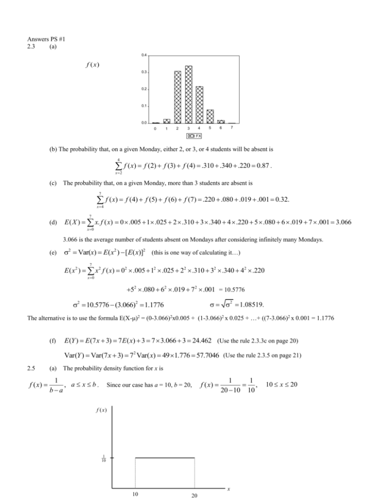
Answers PS #1
2.3
(a)
0.4
f ( x)
0.3
0.2
0.1
0.0
0
1
2
5
4
3
7
6
FX
(b) The probability that, on a given Monday, either 2, or 3, or 4 students will be absent is
4
 f ( x)  f (2)  f (3)  f (4)  .310  .340  .220  0.87 .
x2
(c)
The probability that, on a given Monday, more than 3 students are absent is
7
 f ( x)  f (4)  f (5)  f (6)  f (7)  .220  .080  .019  .001  0.32.
x4
7
(d)
E ( X )   x. f ( x)  0  .005  1 .025  2  .310  3  .340  4  .220  5  .080  6  .019  7  .001  3.066
x 0
3.066 is the average number of students absent on Mondays after considering infinitely many Mondays.
(e)
2  Var(x)  E( x2 )  [ E( x)]2 (this is one way of calculating it…)
7
E ( x 2 )   x 2 f ( x)  02  .005  12  .025  22  .310  32  .340  42  .220
x 0
52  .080  62  .019  72  .001 = 10.5776
  2  1.08519.
2  10.5776  (3.066)2  1.1776
The alternative is to use the formula E(X-)2 = (0-3.066)2x0.005 + (1-3.066)2 x 0.025 + …+ ((7-3.066)2 x 0.001 = 1.1776
(f)
E (Y )  E (7 x  3)  7 E ( x)  3  7  3.066  3  24.462 (Use the rule 2.3.3c on page 20)
Var(Y )  Var(7 x  3)  72 Var( x)  49 1.776  57.7046 (Use the rule 2.3.5 on page 21)
2.5
f ( x) 
(a)
The probability density function for x is
1
, a  x b.
ba
Since our case has a = 10, b = 20,
f ( x) 
1
1
 ,
20  10 10
f ( x)
1
10
x
10
20
10  x  20
(b) The total area beneath the pdf for 10  x  20 is the area of a rectangle. Namely,
Area = (20  10) 
(c)
2.6
1
1
10
P(17  X  19)  (19  17) 
1
 0.2
10
(a) For 4-year schools
P(men and 4-year) 
4,076,416
 0.27
15,064,859
P(women and 4-year) 
4,755,790
 0.32
15,064,859
(b) Let
X=0
if a male is selected
X=1
if a female is selected
Y=1
if 4-year student is chosen
Y=2
if 2-year student is chosen
Y=3
if a less than 2-year student is chosen
P( X  0)  P( X  0, Y  1)  P( X  0, Y  2)  P( X  0, Y  3)
 0.27  0.16  0.01  0.44
P(Y  2)  P( X  0, Y  2)  P( X  1, Y  2)  0.16  0.22  0.38
(c) For f ( x), we note from part (b) that f (0)  0.44. Similarly, for f (1) we obtain
f (1)  P( X  1)  0.32  0.22  0.02  0.56
Thus, the marginal probability function f ( x) is given by
0.44 for x  0
f ( x)  
0.56 for x  1
For g ( y ) we have
0.27  0.32  0.59 for y  1

g ( y )  0.16  0.22  0.38 for y  2
0.01  0.02  0.03 for y  3

(d) The conditional probability function for Y given that X = 1 can be obtained using the result
P(Y  y X  x) 
Thus,
P(Y  y, X  x) f ( x, y)

P( X  x)
f ( x)
0.32 0.56  0.57 for y  1

f ( y x  1)  0.22 0.56  0.39 for y  2
0.02 0.56  0.04 for y  3

(e) If a randomly chosen student is male, the probability that he attends a 2-year college is
P(Y  2 X  0) 
P(Y  2, X  0) .16

 .36
P( X  0)
.44
(f) If a randomly chosen student is a male, the probability that he attends either a 2-year college or a 4-year
college is
P(Y  1 or Y  2 X  0)  P(Y  1 X  0)  P(Y  2 X  0)

P(Y  1, X  0) P(Y  2, X  0)

P( X  0)
P( X  0)

.27 .16

 .61  .36  .97
.44 .44
(g) For gender and type of college institution to be statistically independent, we need
f ( x, y )  f ( x ) g ( y )
for all x and y.
For x = 0 and y = 1, we have
f (0,1)  0.27  f (0) g (1)  0.44  0.59  0.26
While these two values are close, they are not identical. Hence, gender and type of institution are not
independent.
2.7
The mutual fund has an annual rate of return, X ~ N (0.1,0.042 ) .
For each one of these problems, sketch a diagram of the normal curve and SHADE in the area that corresponds to the question.
Then use the normal probability table to determine the actual area.
(a)
0  0.1 

P( X  0)  P z 
  p( z  2.5)  0.5  0.4938  0.0062
0.04 

(b)
0.15  0.1 

P( X  0.15)  P z 
  P( z  1.25)  0.5  0.3944  0.1056
0.04 

(c)
Now, X ~ N (0.12,0.052 )
0  0.12 

P( X  0)  P z 
  p( z  2.4)  0.5  0.4918  0.0082
0.05 

0.15  0.12 

P( X  0.15)  P z 
  P( z  0.6)  0.5  0.2257  0.2743
0.05 

From the modification, the probability that a 1-year return will be negative is increased from 6.2% to 8.2%, and the
probability that a 1-year return will exceed 15% is increased from 10.56% to 27.43%. Since the chance of negative
return has increased only slightly, and the chance of a return above 15% has increased considerably, I would advise
the fund managers to make the portfolio change.
2.9
2.12
not on list, but still good practice. Draw a normal distribution for each one of these and shade in the appropriate
area:
(a)
P(Z  3)  P(Z  0)  P(0  Z  3)  .5  .4987  0.9987
(b)
P(Z  1)  P(Z  0)  P(0  Z  1)  .5  .3413  0.8413
(c)
P( z  1)  P( z  0)  P(1  z  0)  0.5  0.3413  0.1587
(d)
P( z  3)  P( z  0)  P(3  z  0)  0.5  0.4987  0.0013
(e)
P(1  Z  1)  2  P(0  Z  1)  .3413  2  .6826
(f)
P(3  z  1)  P(3  z  0)  P(0  z  1)  0.4987  0.3413  0.84
(g)
Computer software files xr2-9.xls, contain the instructions for computing these probabilities.
(a)
2 x 0  x  1
f  x  
otherwise
0
f(x)
2
1
(b)
x
P(0  X  21 )  21 ( 21 )(1)  41 (this is the area under the line above from X=0 to X=1/2. Shade this area in on the
graph. To calculate the area, remember that the area of a triangle is (1/2)*base*height.)
(c)
P( 14  X  34 )  P( X  34 )  P( X  14 )  12 ( 34 )( 32 )  12 ( 14 )( 12 )  169  161  12
(this is the area
under the line above between X=1/4 and X=3/4. shade your graph…i can’t seem do shade in Word)
2.14
The joint probability density function for the random variables, gender (G) and political affiliation (P), is
G
P
0
1
2
0
.20
.30
.06
The marginal probability density functions are
1
.27
.10
.07
0.44 if g  0
f g  
0.56 if g  1
0.47 if

f  p   0.40 if
0.13 if

and
p0
p 1
p2
(a) For the two random variables, G and P, to be independent,
f  g , p  f  g  f  p 
When g = 0 and p = 0, we have f (0,0) = 0.27. However, f ( g  0) = 0.44 and f ( p  0) = 0.47. Thus,
f ( g  0). f ( p  0) = 0.44  0.47 = 0.2068  0.27 = f (0,0) . Hence the random variables P and G are not
independent. Similarly, f (11
, ) = 0.3, f ( g  1) = 0.56 and f ( p  1) = 0.4. Again 0.3  0.56  0.4,
providing further evidence that the two random variables G and P are not independent.
(b)
f  g, p 
f  p | G  1 
f  g  1
. Thus we can set up the following table.
f  g , p
p
f  x  p x 1  p
2.15
f  p G  1
f  g  1
0
0.20
0.56
0.3571
1
0.30
0.56
0.5357
2
0.06
0.56
0.1071
1 x
for x = 0,1.
(a) The mean of the discrete random variable, X, is
E  X    x f  x   0  f  0   1 f 1  p1 1  p 
11
p
x
The variance of X is
 2  var  X   E  X  E  X     x  p f  x     x  p p x 1  p
2
2
2
x
   p p 0 1  p
2
1 0
 1  p p 1 1  p
2
1 x
x
11
 p 2 1  p  1  p p  p1  p p  1  p  p1  p
2
(b) E[ B]  E[ X 1  X 2 ... X n ]  E[ X 1 ]  E[ X 2 ]  ...  E[ X n ]  p  p  p  np
Given X 1 , X 2 ,..., X n are independent, we have
var  B  var  X 1  X 2 ... X n   var  X 1   var  X 2 ... var  X n 
 p1  p  p1  p... p1  p  np1  p
(c)
np
B 1
E[Y ]  E    E[ B] 
p
n
n n
np1  p p1  p
 B 1
var Y   var    2 var  B 

 n n
n
n2
2.16
2
4
6
X
1
Y
3
9
1/8
1/4
1/8
1/2
1/24
1/4
1/24
1/3
1/12
0
1/12
1/6
1/4
1/2
1/4
(a) The marginal probability density function of Y is h(y) where
h(1) = 1/2
h(3) = 1/3
h(9) = 1/6
(b) The conditional probability density function for y is given by the equation f ( y | x) 
f ( x, y)
. Applying
f ( x)
this rule, we can obtain f ( y |2) , which is given by
f ( y |2)
y
1
f (2,1) f (2)  (1 / 8) (1 / 4)
= 1/2
3
f (2,3) f (2)  (1 / 24) (1 / 4)
= 1/6
9
f (2,9) f (2)  (1 / 12) (1 / 4)
= 1/3
Therefore, the conditional probability density function, f ( y |2) , is given by
f (1|2) = 1/2
f (3|2) = 1/6
f (9|2) = 1/3
(c) cov X , Y   E[ X  E ( X )][Y  E (Y )]
where E  X   2  41  4  21  6  41  4
E Y   1  21  3  13  9  16  3
From first principles
cov X , Y      x  4 y  3 f  x , y 
x
y
1 
 2  41  3 81  2  43  3 24
1  64 93 1
 6  43  3 24
   12
0
Alternatively, using results in Section 2.5 it is possible to show that
cov X , Y   E[ X  E  X ][Y  E Y ]  E  XY   E  X  E Y 
This is an important result that will be used throughout the text. In terms of the current example we can
show that E(XY) = 12
E(XY) = (2)(1)(1/8) + (2)(3)(1/24) + (2)(9)(1/12)
+ (4)(1)(1/4) + (4)(3)(1/4) + (4)(9)(0)
+ (6)(1)(1/8) + (6)(3)(1/24) + (6)(9)(1/12) = 288/24 = 12
and hence that
cov X , Y   12  4  3  0
(d) This is an example where X and Y are not independent, despite the fact that their covariance is zero. If X
and Y are independent, then f  x, y  g xh y . To prove that this result does not hold let us consider
two outcomes. First, if x = 2 and y = 3,
f 2,3 
1
24
 g2h3 
1
 
1
1
4
3
12
Also, if x = 4 and y = 9
f 4,9  0  g4h9 
2.23
1

2
1
6
1

12
(a) f 0,0  0.6 0.4 0.3 052
.  2 0  0.208
0
1
0
1
f 0,1  (0.6) 0 0.4 0.3 0.52 2 0  0120
.
1
1
0
f 1,0  0.6 0.4 0.3 0.52 2 0  0.312
1
0
0
1
f 11
,   0.6 0.4 0.3 0.52 2 1  0.360
1
0
1
0
X\Y
0
1
0
0.208
0.120
0.328
1
0.312
0.360
0.672
0.52
0.48
1.0
(b)
(c)
By summing the relevant values we obtain these marginal distributions
x
f  x
y
f  y
0
1
0.328
0.672
0
1
0.52
0.48
This function is given by f  y | x  0  
y
f 0, y 
f  0, y 
f  x  0
f  x  0
f  y | x  0
0
0.208
0.328
0.6341
1
0120
.
0.328
0.3659
(d)
E[ X ]   x f  x   0.672
x
(e)
E[Y ]   y f  y   0.48
y
(f)
E[ X 2 ]   x 2 f  x   0.672
x
var X   E[ X 2 ]  [ E  X ]2  0.672  0.672  0.2204
2
E [Y 2 ]   y 2 f  y   0.48
y
var Y   0.48  0.48  0.2496
2
E[ XY ]    xy f  x , y   0.36 this is the term (1)(1)(0.36) = 0.36
x
y
(This sum has four terms but three of the four involve zero values, leaving only one of the four terms being nonzeroOnly the terms where both x and y are equal to one needs to be considered in the above summation. Other terms
are zero.)
cov X , Y   E [ XY ]  E [ X ]E [Y ]  0.36  0.6720.48  0.03744

(g)
cov X , Y 
var  X  var Y 

0.03744
0.22040.2496
 01596
.
Use the rules on page 31:
E[ X  Y ]  E[ X ]  E[Y ]  0.672  0.48  1152
.
var X + Y   var X   varY   2 cov X , Y 
 0.2204  0.2496  20.03744  0.5449
2.25
Let X represent the life length of the computer. The fraction of computers lasting for a given time is equal to the
probability of one computer, selected at random, lasting for that given time. For each probability below, you should draw
a picture of the normal distribution and shade in the area that corresponds to the question. Then, standardize the value and
use the table to determine the probability (area).
(a)
1  2.9 

P X  1  P Z 
.   0.5  P0  Z  1357
.   0.5  0.413  0.087
  P Z  1357

196
. 
(b)
4  2.9 

P X  4  P Z 
  P Z  0.786  0.5  P0  Z  0.786  0.5  0.284  0.216

14
. 
(c)
2  2.9 

P X  2  P Z 
  P Z  0.643  0.5  P0  Z  0.643  0.5  0.240  0.740

14
. 
(d)
4  2.9 
 2.5  2.9
P2.5  X  4  P
Z
  P 0.286  Z  0.786
 14
.
14
. 
 P 0.286  Z  0  P0  Z  0.786  0112
.
 0.284  0.396
(e)
We want X0 such that P(X < X0) = 0.05. Now, P(0 < Z < 1.645) = 0.45 (from tables). Hence, P(Z < 1.645) = 0.05.
Thus, an appropriate X0 is defined by
1645
.

2.26 NOTE: skip this one…
X 0  2.9
. 14
.   0.6.
or X 0  2.9  1645
14
.