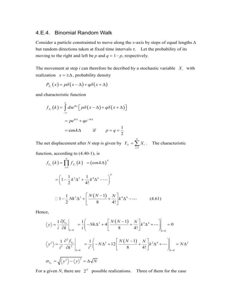
4.E.4. Binomial Random Walk
Consider a particle constrainted to move along the x-axis by steps of equal lengths Δ
but random directions taken at fixed time intervals τ. Let the probability of its
moving to the right and left be p and q  1 p, respectively.
The movement at step i can therefore be decribed by a stochastic variable X i with
realization x   , probability density
PXi  x   p  x     q  x   
and characteristic function
f Xi  k  

 dxe
 p  x     q  x   
ikx

 peik   qeik 
 cosk 
if
pq
1
2
N
The net displacement after N step is given by YN   X i . The characteristic
i 1
function, according to (4.40-1), is
N
fYN  k    f X i  k    cos k  
N
i 1
1
 1
 1  k 22  k 4 4 
4!
 2



N
 N  N  1 N  4 4
1
1  Nk 2 2  
 k  
2
8
4! 

(4.61)
Hence,
y 
y
2
k 0
2
1  fYN
 2
i k 2
Y 
N
1 fYN
i k
 N  N  1 N  3 4
1
   Nk  2  4 
 k  
i 
8
4! 


k 0
y2  y
2

  0
 k 0
 N  N  1 N  2 4
1
 N  2  12 
 k  
2 

i 
8
4! 


2
  N 
 k 0
 N
For a given N, there are 2 N possible realizations. Three of them for the case
N  2000 are shown in Fig.4.4.
Differential Equation
Consider the limits ,  0 with N   .
Setting fY  k , N   fYN  k  , we have
fY k ,  N  1   fY  k , N    cos k  
  cos k   1 cos k  
N 1
  cos k  
N
N
1
 1
   k 22  k 44 
4!
 2
Hence, with N  t , we have

 fY  k , N 

(4.62)
fY  k , t 
f  k , t     fY  k , t 
 lim Y


0
t

 lim
fY k ,  N  1   fY  k , N 
 0

 1 2 2 1 4 4
 lim   k
 k

 0
 4! 
 2
  Dk 2 fY  k , t 
(4.63)

 fY  k , t 

as   0
(4.64)
where the diffusion coefficient D is defined as
2
D  lim
 , 0 2
For a fixed k, the general solution to (4.64) is
fY  k , t   fY  k ,0  exp   Dk 2t 
 exp   Dk 2t 
if
fY  k ,0  1
(4.66)
Taking the inverse Fourier transform gives the probability distribution
P  y, t  

 2 exp  iky  Dk t 
dk
2

2

 y 2   dk
iy  

 exp  
exp   Dt  k 

 
2 Dt  


 4 Dt   2
 y2 
exp  

4 Dt
 4 Dt 
1

(4.67)
which is a Gaussian with   2Dt .
Alternative Derivation
Consider the stochastic variable Z N 
YN
. The associated characteristic
 N
function , according to (4.40-1), is
N 

 ik

f Z N  k      dx j exp 
x j  PX j  x j 
 N 
j 1  

N

j 1
k 
 k 

fX j 
   cos

N
 N 


k2
k4
1




2
 2 N 4! N



N
(4.68)
N
Hence
 k2 
f Z  k   lim f Z N  k   exp   
N 
 2
PZ  z  


dk
1
 2 exp  ikz  2 k

2
(4.69)



 z 2   dk
2
 1
 exp    
exp    k  iz  
 2

 2   2

 z2 
1
exp   

 2
For very large N, we have PZ N  z 
PYN  y 

 dz  y  

N z PZ  z 


1
 N


 dz  z  

PZ  z  so that from (4.49), we have
y
N

 PZ  z 



y2 
exp   2 
 2 N
 2 N 
1
(4.70)
If the partical takes n per unit time, we have N  nt . Setting D 
P  y, t   lim PYN  y 
N 
See Fig.4.5.
 y2 

exp  

4 Dt
 4 Dt 
1
(4.71)
1 2
n , we have
2