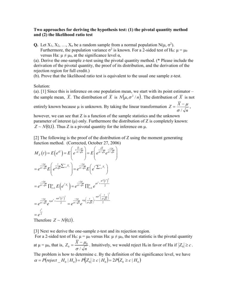
Two approaches for deriving the hypothesis test: (1) the pivotal quantity method
and (2) the likelihood ratio test
Q. Let X1, X2, …, Xn be a random sample from a normal population N(μ, σ2).
Furthermore, the population variance σ2 is known. For a 2-sided test of H0: μ = μ0
versus Ha: μ ≠ μ0, at the significance level α,
(a). Derive the one-sample z-test using the pivotal quantity method. (* Please include the
derivation of the pivotal quantity, the proof of its distribution, and the derivation of the
rejection region for full credit.)
(b). Prove that the likelihood ratio test is equivalent to the usual one sample z-test.
Solution:
(a). [1] Since this is inference on one population mean, we start with its point estimator –
the sample mean, X . The distribution of X is N  ,  2 / n  . The distribution of X is not
X 
entirely known because μ is unknown. By taking the linear transformation Z 
,
/ n
however, we can see that Z is a function of the sample statistics and the unknown
parameter of interest (μ) only. Furthermore the distribution of Z is completely known:
Z ~ N 0,1 . Thus Z is a pivotal quantity for the inference on μ.
[2] The following is the proof of the distribution of Z using the moment generating
function method. (Corrected, October 27, 2006)
 t X  
 tX t  
tZ
/ n
M Z t   E e  E  e
  E  e / n e / n 








n
t
t
t 
n

 i1 X i   / n  t*  i1 X i 
 e / n E  e n
E e
  e






 
e
t
/ n
 
in1 E et X i  e
*
e
 
n t
t
n t * 
/ n
2
2
e
t
* 2
e
t
/ n
t
/ n
e
in1 e
t* 
 
 2 t*
2
2
 t 
n 2 

 t 
 n 
n 


2
 n 
2
2
e2
Therefore Z ~ N 0,1 .
[3] Next we derive the one-sample z-test and its rejection region.
For a 2-sided test of H0: μ = μ0 versus Ha: μ ≠ μ0, the test statistic is the pivotal quantity
X  0
at μ = μ0, that is, Z 0 
. Intuitively, we would reject H0 in favor of Ha if Z 0  c .
/ n
The problem is how to determine c. By the definition of the significance level, we have
  Preject _ H 0 | H 0   P Z 0  c | H 0   2PZ 0  c | H 0 
Thus  / 2  PZ 0  c | H 0  and subsequently we have c  z / 2
That is, at the significance level α, we reject H0 in favor of Ha if Z0  z / 2 .
(b). For a 2-sided test of H0: μ = μ0 versus Ha: μ ≠ μ0, when the population is normal and
population variance σ2 is known, we have:
   ,  2  :    0 ,  2   2  and    ,  2  :     ,  2   2 
The likelihoods are:
L   L0 ,  2   i 1
n
n
 xi  0 2   1  2
 1

exp  
exp 

2
2
2

2
 2
2 2

  2 
1
 x
n
i 1
i
2
 0  

There is no free parameter in L  , thus Lˆ   L  .
n
 xi   2   1  2
n
 1



xi   2 


L   L  ,   i 1
exp  
exp 
2
2 
2 i 1

2
2
 2

2

  2 
There is only one free parameter μ in L . Now we shall find the value of μ that
n
n
1
xi   2 .
maximizes the log likelihood ln L    ln 2 2  
2 i 1
2
2
n
d ln L  1
By solving
 2 i 1 xi     0 , we have ̂  x
d

It is easy to verify that ̂  x indeed maximizes the loglikelihood, and thus the
likelihood function.
1
n
2
Therefore the likelihood ratio is:
n
2
n


 1
xi  0 2 
exp  

2 
2 i 1
L 0 ,  
L 0 ,    2 
Lˆ 
2







n
2
2
ˆ
ˆ




max
L

,

L

,

L

n
 1 2
 1
xi  x 2 
exp  

2 
2 i 1
 2 
 2

1
2
2
 
 1
 exp 
2
 2
 x
n
i 1
  0    xi  x 
2
i
2
 1  x  0  2 

 1
2
   exp   z0  
  exp   

 2

 2   / n  

Therefore, the likelihood ratio test that will reject H0 when   * is equivalent to the ztest that will reject H0 when Z 0  c , where c can be determined by the significance level
α as c  z / 2 .