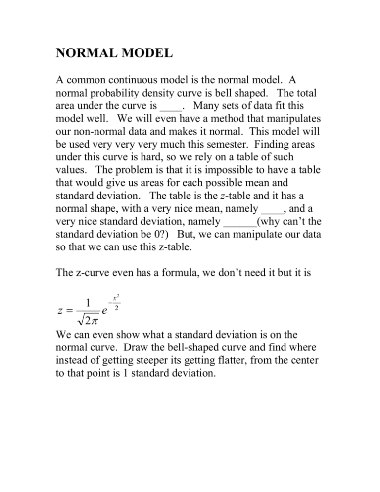
NORMAL MODEL
A common continuous model is the normal model. A
normal probability density curve is bell shaped. The total
area under the curve is ____. Many sets of data fit this
model well. We will even have a method that manipulates
our non-normal data and makes it normal. This model will
be used very very very much this semester. Finding areas
under this curve is hard, so we rely on a table of such
values. The problem is that it is impossible to have a table
that would give us areas for each possible mean and
standard deviation. The table is the z-table and it has a
normal shape, with a very nice mean, namely ____, and a
very nice standard deviation, namely ______(why can’t the
standard deviation be 0?) But, we can manipulate our data
so that we can use this z-table.
The z-curve even has a formula, we don’t need it but it is
z
1
e

x2
2
2
We can even show what a standard deviation is on the
normal curve. Draw the bell-shaped curve and find where
instead of getting steeper its getting flatter, from the center
to that point is 1 standard deviation.
We would like you to know how much of data from a
normal distribution is within +/- 1 standard deviation from
the mean. Can you estimate from the picture?
We would like you to know how much of data from a
normal distribution is within +/- 2 standard deviations from
the mean as well as +/- 3 standard deviations from the
mean. Can you estimate these from the picture?
By the way we can give some info about the same
questions for ANY distribution (even the wackiest one you
can come up with). The following table summaries:
Standard Dev’s from mean Normal case ANY case
+/- 1
Approx 68% 0%-100%
+/- 2
Approx 95% 75%-100%
+/- 3
Approx 99.7% 88.8%-100%
How to use the z-table for any normal X:
Let X be normal with mean  and standard deviation
.
As an example consider a test with a mean of 55 and a
standard deviation of 10 and a normal shape to the scores.
Recall our rules for RV’s
x-55 will have _________shape with a mean of _______
and a standard deviation of __________
(x-55)/10 will have __________shape with a mean of
_______ and a standard deviation of __________
In general:
Step 1: Make a new RV that is X – 
This RV has mean ______ and standard deviation ______
and shape ________

Step 2: Make a new RV that is (X –  ) /
This RV has mean _____ and standard deviation ________
And shape _________
This last RV is so great we give it a deserving name Z.
Note in the formula X is the original RV, and Z is called its
standardized version:
x  mean
z
st .deviation
If you take just one piece of data x and find the
corresponding z it gives you how many standard deviations
from the mean the x is and in which direction. Example: if
you have an x of 15 and the mean is 9 and the standard
deviation is 2, then 15 is 3 standard deviations above the
mean and sure enough z=(15-9)/2 = 3.
A z-score is useful because it helps us describe and
compare data in a universal language. Example: which is
more extreme? A rat that weighs 3 lbs or an elephant that
weighs 11100 lbs? Suppose that rats mean weight is 1 lb
with a standard deviation of .5 lbs and that for elephants the
mean is 11000 lbs and the standard deviation is 1000 lbs.
Well 11100 lbs is certainly a lot more than 3 lbs, but of
course this is not a fair comparison to say the elephant is
more extreme. The elephant is 100 lbs more than the
average, while the rat is only 2 lbs more, but again this is
not fair. The way to make a comparison is to find the z –
score of each (how many standard deviations from the
mean).
Note that when using the formula:
x  mean
z
st .deviation
the data doesn’t have to be normal.
Example: Suppose the heights of young women have a
normal distribution with a mean of 64 inches and a standard
deviation of 2.7 inches. Pick a young woman at random
and find her height and let the outcome of this random
variable be X.
Find P(68≤X≤70)
Find P(X>66)
What heights make up the tallest 10%?
What heights make up the shortest 20%?
Find the area from z = -1.00 to 1.00.
Find the area from z = -2.00 to 2.00.
Notice these areas correspond to the 68% and 95% we
mentioned in the table telling how much data is within 1, 2,
and 3 standard deviations from the mean when dealing with
the normal curve.
The height problem above was done assuming a normal
model and hence that people report their heights with
infinite accuracy. Suppose that people only worry about
their heights to the nearest inch. If so P(68≤X≤70) would
probably be higher than what we got earlier. Why?
We won’t worry about this problem in general, but to get a
more accurate answer we should find out how accurate the
measurements are and go +/- half that accuracy on either
side to get a better approximation than just assuming an
exact normal curve.