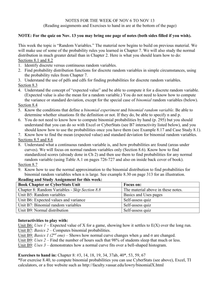
NOTES FOR THE WEEK OF NOV 6 TO NOV 13
(Reading assignments and Exercises to hand in are at the bottom of the page)
NOTE: For the quiz on Nov. 13 you may bring one page of notes (both sides filled if you wish).
This week the topic is “Random Variables.” The material now begins to build on previous material. We
will make use of some of the probability rules you learned in Chapter 7. We will also study the normal
distribution in much greater detail than in Chapter 2. Here is what you should learn how to do:
Sections 8.1 and 8.2
1. Identify discrete versus continuous random variables.
2. Find probability distribution functions for discrete random variables in simple circumstances, using
the probability rules from Chapter 7.
3. Understand the use of pdfs and cdfs for finding probabilities for discrete random variables.
Section 8.3
4. Understand the concept of “expected value” and be able to compute it for a discrete random variable.
(Expected value is also the mean for a random variable.) You do not need to know how to compute
the variance or standard deviation, except for the special case of binomial random variables (below).
Section 8.4
5. Know the conditions that define a binomial experiment and binomial random variable. Be able to
determine whether situations fit the definition or not. If they do, be able to specify n and p.
6. You do not need to know how to compute binomial probabilities by hand (p. 295) but you should
understand that you can do so with Excel or CyberStats (see B7 interactivity listed below), and you
should know how to use the probabilities once you have them (see Example 8.17 and Case Study 8.1).
7. Know how to find the mean (expected value) and standard deviation for binomial random variables.
Sections 8.5 and 8.6
8. Understand what a continuous random variable is, and how probabilities are found (areas under
curves). We will focus on normal random variables only (Section 8.6). Know how to find
standardized scores (already done in Ch 2) and then use them to find probabilities for any normal
random variable (using Table A.1 on pages 726-727 and also on inside back cover of book).
Section 8.7
9. Know how to use the normal approximation to the binomial distribution to find probabilities for
binomial random variables when n is large. See example 8.30 on page 313 for an illustration.
Reading and Study Assignment for this week:
Book Chapter or CyberStats Unit
Focus on:
Chapter 8: Random Variables - Skip Section 8.8
The material above in these notes.
Unit B5: Random variables
Basics and Uses pages
Unit B6: Expected values and variance
Self-assess quiz
Unit B7: Binomial random variables
Self-assess quiz
Unit B9: Normal distribution
Self-assess quiz
Interactivities to play with:
Unit B6: Uses 1 – Expected value of X for a game, showing how it settles to E(X) over the long run.
Unit B7: Basics 2 – Computes binomial probabilities.
Unit B9: Basics 1 (2nd one) – Shows how normal curve changes when µ and σ are changed.
Unit B9: Uses 2 – Find the number of hours such that 98% of students sleep that much or less.
Unit B9: Uses 3 – demonstrates how a normal curve fits over a bell-shaped histogram.
Exercises to hand in: Chapter 8: #3, 14, 18, 19, 34, 37ab, 40*, 53, 59, 67
*For exercise 8.40, to compute binomial probabilities you can use CyberStats (see above), Excel, TI
calculators, or a free website such as http://faculty.vassar.edu/lowry/binomialX.html