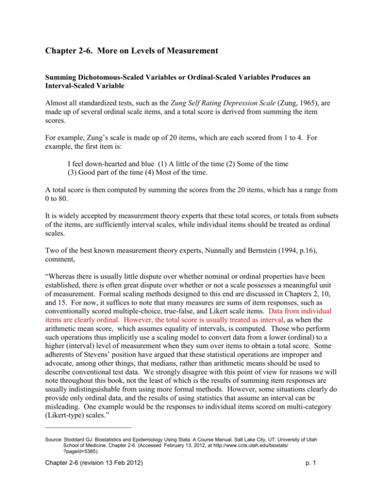
Chapter 2-6. More on Levels of Measurement
Summing Dichotomous-Scaled Variables or Ordinal-Scaled Variables Produces an
Interval-Scaled Variable
Almost all standardized tests, such as the Zung Self Rating Depression Scale (Zung, 1965), are
made up of several ordinal scale items, and a total score is derived from summing the item
scores.
For example, Zung’s scale is made up of 20 items, which are each scored from 1 to 4. For
example, the first item is:
I feel down-hearted and blue (1) A little of the time (2) Some of the time
(3) Good part of the time (4) Most of the time.
A total score is then computed by summing the scores from the 20 items, which has a range from
0 to 80.
It is widely accepted by measurement theory experts that these total scores, or totals from subsets
of the items, are sufficiently interval scales, while individual items should be treated as ordinal
scales.
Two of the best known measurement theory experts, Nunnally and Bernstein (1994, p.16),
comment,
“Whereas there is usually little dispute over whether nominal or ordinal properties have been
established, there is often great dispute over whether or not a scale possesses a meaningful unit
of measurement. Formal scaling methods designed to this end are discussed in Chapters 2, 10,
and 15. For now, it suffices to note that many measures are sums of item responses, such as
conventionally scored multiple-choice, true-false, and Likert scale items. Data from individual
items are clearly ordinal. However, the total score is usually treated as interval, as when the
arithmetic mean score, which assumes equality of intervals, is computed. Those who perform
such operations thus implicitly use a scaling model to convert data from a lower (ordinal) to a
higher (interval) level of measurement when they sum over items to obtain a total score. Some
adherents of Stevens’ position have argued that these statistical operations are improper and
advocate, among other things, that medians, rather than arithmetic means should be used to
describe conventional test data. We strongly disagree with this point of view for reasons we will
note throughout this book, not the least of which is the results of summing item responses are
usually indistinguishable from using more formal methods. However, some situations clearly do
provide only ordinal data, and the results of using statistics that assume an interval can be
misleading. One example would be the responses to individual items scored on multi-category
(Likert-type) scales.”
_______________________
Source: Stoddard GJ. Biostatistics and Epidemiology Using Stata: A Course Manual. Salt Lake City, UT: University of Utah
School of Medicine. Chapter 2-6. (Accessed February 13, 2012, at http://www.ccts.utah.edu/biostats/
?pageId=5385).
Chapter 2-6 (revision 13 Feb 2012)
p. 1
A refinement of this idea
Although summing individual items to produce an interval scale is widely accepted, a little
thought will make you wonder.
For example, suppose you provide the following list of tasks for someone putting weight (post
weightbearing) on a leg after a hip replacement operation:
1.
2.
3.
4.
5.
Stand up from a sitting position
Walk from room to room in own house using a cane or walker
Walk from room to room in own house unassisted
Walk up one flight of stairs
Run on treadmill for 5 minutes
If you sum up the number of tasks completed to get a total score, is it really an interval scale?
The problem is that the tasks do not have the same level of difficultly, so the sum will not strictly
have equal intervals. To make this a true interval scale, you need to weight the items by level of
difficultly. An excellent way to assign weights is the Rasch Model, which is popularly used in
measurement development. An excellent textbook on applying this method is Bond and Fox
(2007).
In referring to the common practice of scoring the number of items correctly answered on a test
in school, such as a math test, or going on to express this as a percentage, to measure the
student’s ability, Bond and Fox (2007, p.21) regard this as only an ordinal scale,
“…The routine procedure in education circles is to express each of these n/N fractions as
a percentage and to use them direcly in reporting students’ results. We will soon see that
his commonpalce procedure is not justified. In keeping with the caveat we expressed
earlier, these n/N fractions should be regarded as merely orderings of the nominal
categories, and as insufficient for the inference of interval relations between the
frequencies of observations.”
Bond and Fox (2007) then go on to show how to weight the difficulty of the exam questions
using a Rasch Model to provide a true interval scale with equal intervals of difficulty or student
ability.
Chapter 2-6 (revision 13 Feb 2012)
p. 2
Visual Analog Scales for Symptom Measurements
A frequently used way to assess pain is the visual analog scale (VAS). Here, the study subjects
rates his or her pain by placing a mark on a visual scale, such as,
|--------------------------------------------------------------|
no
pain
worst
possible
pain
These are frequently drawn with a line 100 mm long, so the score is the mm distance from the
left (range, 0 to 100). Another variation is an integer rating, from 0 to 10.
In remarking on what level of measurement such a scale achieves, McDowell (2006, p.478), in
his textbook on rating scales, comments without commiting himself to an opinion,
“Although nonparametric statistical analyses are generally considered appropriate (4),
one study showed that VAS measures produced a measurement with ratio scale properties
(12).”
-------------(4) Huskisson EC. (1982). Measurement of pain. J Rheumatol 9;768-769.
(12) Price DD, McGrath PA, Rafi A, et al. (1983). The validation of visual analogue
scales as ratio scale measures for chronic and experimental pain. Pain 17:45-56.
Perhaps the best article to cite for justifying that a VAS can be analyzed as an interval scale is
Dexter and Chestnut (1995). These authors did a Monte Carlo simulation, sampling from an
actual VAS dataset, and demonstrated that the independent sample t-test (assumes interval scale)
performed as well as the Wilcoxon-Mann-Whitney test (assumes ordinal scale) in not inflating
the Type I error rate. Similarly, they showed the oneway analysis of variance (assumes interval
scale) performed as well as the Kruskal-Wallis test (assumed ordinal scale) in not inflating the
Type I error rate. So, treating the VAS as an interval scale for analysis resulted in a correct
hypothesis test.
In their methods paper assessing the bias and precision of VAS’s, Paul-Dauphin et al (1999)
analyze these scales using a statistical approach that assumes at least an interval scale. These
authors discuss the different approaches of expressing the VAS, such as reference ticks and
labels or not, vertical versus horizontal. It is a good paper to cite if you intend to use a VAS, if
you want to show you have put some effort into designing your study well.
Chapter 2-6 (revision 13 Feb 2012)
p. 3
How Many Categories In An Ordinal Scale Are Required To Consider It an Interval Scale
It would seem that adding more categories would take an ordinal scale closer to an interval scale,
regardless of whether the intervals are strictly equal sized or not. This occurs because with more
categories, there is less opportunity for the intervals to have large inequalities.
Also, an ordinal scale has an underlying theoretical continuous scale. So, the scores of the
ordinal scale are approximations of the underlying continuous scale. It is somewhat analogous to
expressing height by rounding to the nearest inch or centimeter.
So, just how many categories does it take for justifying analyzing an ordinal scale as an interval
scale?
Nunnally and Bernstein (1994, p.115) make a suggestion about the number of categories,
“We will somewhat arbitrarily treat a variable as continuous if it provides 11 or more
levels, even though it is not continuous in the mathematical sense. Consequently we will
normally think of item responses as discrete and total scores as continuous. The number
11 is not ‘magical,’ but experience has indicated that little information is lost relative to a
greater number of categories. Moreover, the law of diiminishing returns applies, and so
using even 7 or 9 categories does little harm if the convenience of reporting data as a
single digit is improtant to the application.”
Exercise. Download the Multiple Sclerosis Quality of Life (MSQOL)-54 Instrument from the
website: http://gim.med.ucla.edu/FacultyPages/Hays/MSQOL-54%20instrument.pdf
Go to items 53 and 54 on the second to last page. Item 53 is a 11 point scale and item 54 is a 7
point scale. Which would you say does the best job of approaching the accuracy of an interval
scale?
Chapter 2-6 (revision 13 Feb 2012)
p. 4
Is It All Right to Treat an Ordinal Scale as an Interval Scale for Analysis?
Point
Actually it is okay to analyze an ordinal scale using statistical methods that require an interval
scale, but do not do it, since the idea has not yet caught on in biomedicine. You can, however,
use this idea to make yourself feel comfortable analyzing sums of items not developed using the
Rasch method as interval scales, or using VAS scales as interval level scales.
Detail (if you are curious)
As explained by Nunnally and Bernstein (1994, p.20), there is one camp, called the
“fundamentalists”, who hold that ordinal scales should strictly be analyzed by the nonparametric
tests that using on the rank order in the data. The other camp, called the “representationalists”
advocated that the essential information in an interval scale is the rank ordering, and that there is
little harm in analyzing ordinal data using parametric tests that assume an interval scale. These
points of view were hotly debated in the 1950s in the social science literature. Studies were done
that demonstrated there was little difference in outcomes by treating an interval scale as an
ordinal scale, either approach produced basically the same correlation coefficient and p value.
What came out of that was a justification for many social science researchers to analyze ordinal
scales as interval scales.
The trend was not adopted by researchers in biomedicine. Most of the measurements in
medicine are either dichotomous or interval, so the issue did not have to be faced.
In contrast, most of the measurements in the social sciences are ordinal, or multiple ordinal items
deriving a total score of a scale. Therefore, the social scientists looked into this question in
ernest, to enable themselves to use regression models and their variants.
A famous biostatistician, Ralph D’Agostino, introduced some papers to introduce the idea into
biostatistics. In his first paper (Heeren and D’Agostino, 1987), it was demonstrated by
simulation that analyzing ordinal scales with a few categories with a t test, and with small sample
sizes, 5 to 20, had the desired statistical property of the type I error being what it should be.
In a followup paper, Sullivan and D’Agostino (2003) investigate the performance of analysis of
covariance, a parametric technique that assumes an interval scale, on ordinal data with 3, 4 and 5
categories. Again, they discovered the type I error was not inflated, while power of the test
remained high.
D’Agostino did not take a position by stating a conclusion for or against analyzing ordinal scaled
data with interval-level statistical approaches. Instead, he published his papers to lay the
groundwork to move biostatisticians in this direction. His work, however, implies that this could
be done and the idea will slowly catch on.
Chapter 2-6 (revision 13 Feb 2012)
p. 5
Dichotomous Variables Are Actually Interval Scaled Variables
Hardly anyone knows this, because it is not taught in statistics courses, but a dichotomous scale
is also an interval scale.
What statistics books will advocate, however, is that categorical variables be converted to a set
of dummy variables, or indicator variables (these are dichotomies, scored 0 or 1), as a way to
include a categorical variable (either nominal or ordinal) into a regression model.
Statistics books fail to point out that the reason this works is that dichotomous variables are
actually interval scales, so arithmetic can be done the variables themselves. Linear regression
estimates an intercept and slope (the equation for a straight line), using the following equations:
n
ˆ1 
n
 ( X i  X )(Yi  Y )
i 1
n
(X
i 1
i
 X)
and
2
ˆ0  Y  ˆ1 X
where X 
X
i 1
i
n
We can see that arithmetic is being done on the variables themselves.
Interval Scale Assumption
Linear regression, as well as the other forms of regression
models, assume that all predictor variables have at least an interval scale.
This assumption is necessary so arithmetic can be performed on the values of each predictor
variable.
It makes sense to do arithmetic on an interval scaled variable, since this scale is
sufficiently close to our notion of integers and real numbers (the interval scale shares the
property of equal intervals with both of these number systems). It is generally accepted that it
does not make sense to do arithmetic on nominal and ordinal scales, since these scales do not
have equal intervals.
Although it is rarely claimed as such, a dichotomous scale could be considered an interval scale,
since it has order (although perhaps an arbitrary order), it has equal intervals (one interval that is
equal to itself), and one category can be selected to represent 0.
This claim is made by Jum C. Nunnally, one of the best-known psychometric experts (Nunnally
and Bernstein, 1994, p.16):
“When there are only two categories, there is only one interval to consider, so that one
interval may be considered an ‘equal’ interval. That is why binary (dichotomous)
variables may be considered to form interval scales, the point noted above as being so
important to modern regression theory and elsewhere in statistics.”
Chapter 2-6 (revision 13 Feb 2012)
p. 6
Nunnally and Bernstein (1994, pp. 189-190) further state:
“As noted in the section titled ‘Another form of Partialling,’ categorical variables are now
used quite commonly in multivariate analysis thanks to Cohen (1968). This use reflects
the point made in Chapter 1 that a scale may be regarded as an interval scale when it
contains only two points. This is the basis of the analysis of variance. If the variable
takes on only two values, such as gender, one level may be coded 0 and the other coded
1…. A variable coded 0 or 1 is called a ‘dummy’ or ‘indicator’ variable. The
independent variable’s ‘scale’ has interval properties, by definition, because the scale has
only two points.”
Sarle (1997), on his web-site discussing measurement theory, states the same thing,
“What about binary (0/1) variables?
For a binary variable, the classes of one-to-one transformations, monotone
increasing/decreasing transformations, and affine transformations are identical--you can't
do anything with a one-to-one transformation that you can't do with an affine
tranformation. Hence binary variables are at least at the interval level. If the variable
connotes presence/absence or if there is some other distinguishing feature of one
category, a binary variable may be at the ratio or absolute level.
Nominal variables are often analyzed in linear models by coding binary dummy
variables. This procedure is justified since binary variables are at the interval level or
higher.”
This is why you can recode nominal and ordinal predictor variables into indicator, or dummy
variables, and include them directly into the regression equation. The regression algorithm treats
the indicator variable as an interval scale, and performs arithmetic directly on the 0-1 values.
This claim that dichotomous variables are actually interval scales is rarely taught in statistics
classes, so few people are even aware why indicator variables work in regression models.
Statisticians are traditionally trained to think of a 0-1 variable as a “Bernoulli variable,” rather
than as a continuous “interval scale” variable. A Bernoulli variable has mean p and variance
p(1-p), where p is the probability of a 1 (Ross, 1998).
The derivation for this mean and variance for a Bernoulli variable, with standard deviation being
the square root of the variance, is taught in the first semester of a masters degree level statistics
program. The important point about the formulas is that they just use the nominal scale property
of the variable. That is, they are based on simply counting the number of occurrences of the
variables outcome (how 0’s and how many 1’s), and then doing arithmetic on the counts.
Arithmetic is not done the values of the variable themselves.
Chapter 2-6 (revision 13 Feb 2012)
p. 7
These formulas for the mean and standard deviation of a Bernoulli variable look very different
than the sample mean and sample standard deviation used in statistics:
n
X 
X
i 1
i
(sample mean)
n
and
n
s  s2 
(X
i 1
i
 X )2
n 1
(sample standard deviation)
Let’s apply these standard formulas to a dichotomous variable and see what happens.
Reading in the Stata formatted data file, births.dta, using Stata menus:
File
Open
Find the directory where you copied the course CD:
Change to the subdirectory datasets & do-files
Single click on births.dta
Open
use births.dta
Chapter 2-6 (revision 13 Feb 2012)
p. 8
Requesting a frequency table for the dichotomous variable, lowbw, using Stata menus:
Statistics
Summaries, tables & tests
Tables
Oneway tables
Categorical variable: lowbw
OK
tabulate lowbw
low birth |
weight |
Freq.
Percent
Cum.
------------+----------------------------------0 |
440
88.00
88.00
1 |
60
12.00
100.00
------------+----------------------------------Total |
500
100.00
We see that the lowbw variable is a 0-1 variable, or Bernoulli variable.
Using the Bernoulli formulas, we get
mean = p = 60/500 = 0.1200
variance = p(1-p) = 0.1200(.8800) = 0.1056
standard deviation =
p(1  p) = .324962
Notice how we just use the counts of the categories, the “Frequency” column of the frequency
table, and then do arithmetic on the counts, rather than the values of the variable. That is, we
computed these test statistics using only the nominal scale property of the variable (we just
counted the frequency of occurrence of the name, or label, given to the variable).
Now, using the ordinary statistical formulas for mean and standard deviation, which were
designed for interval scales,
Statistics
Summaries, tables & tests
Summary and descriptive statistics
Summary statistics
Variables: lowbw
Options: standard display
OK
summarize lowbw
Variable |
Obs
Mean
Std. Dev.
Min
Max
-------------+-------------------------------------------------------lowbw |
500
.12
.325287
0
1
Chapter 2-6 (revision 13 Feb 2012)
p. 9
We see that the Bernoulli mean is exactly the same as when the ordinary formula for the mean is
applied, both giving 0.12.
We see that the Bernoulli standard deviation of 0.324962 does not quite match the ordinary
“sample” standard deviation formula value of 0.325287. However, that is only because the
Bernoulli formula is the population formula. The ordinary “population” formula for the standard
deviation divides by N rather than N-1,
N
  2 
(X
i 1
  )2
i
(population standard deviation)
N
where sigma , ϭ, is the population standard deviation and, mu, µ, is the
population mean.
n 1
, than we have the population standard
n
If we multiply our sample standard deviation by
deviation calculation.
n
n 1
n 1
s
n
n
(X
i 1
i
 X)
n 1
n
2

(X
i 1
i
n
  )2
  , where X is assumed to be equal to 
When we do that,
display 0.325287*sqrt(499)/sqrt(500)
.32496155
which we see is an exact match to the Bernoulli formula, which gave .324962 .
So, treating a dichomous variable as an interval scales works for descriptive statistics.
That is, treating a dichotomous variable as an interval scale and then applying the ordinary
formulas produces an identical result as treating it as a nominal scale Bernoulli variable, and then
applying the Bernoulli formulas.
Next, let’s see what happens with significance tests, seeing if interval scale significance tests
give an identical result to categorical significance tests.
Chapter 2-6 (revision 13 Feb 2012)
p. 10
Computing a t test, using lowbw as the outcome variable, using Stata menus:
Statistics
Summaries, tables & tests
Classical tests of hypotheses
Two-group mean-comparison test
Variable name: lowbw
Group variable name: sex
OK
ttest lowbw , by(sex)
Two-sample t test with equal variances
-----------------------------------------------------------------------------Group |
Obs
Mean
Std. Err.
Std. Dev.
[95% Conf. Interval]
---------+-------------------------------------------------------------------1 |
264
.1022727
.0186842
.3035821
.0654831
.1390624
2 |
236
.1398305
.0226235
.3475482
.0952598
.1844012
---------+-------------------------------------------------------------------combined |
500
.12
.0145473
.325287
.0914185
.1485815
---------+-------------------------------------------------------------------diff |
-.0375578
.0291209
-.0947728
.0196572
-----------------------------------------------------------------------------diff = mean(1) - mean(2)
t = -1.2897
Ho: diff = 0
degrees of freedom =
498
Ha: diff < 0
Pr(T < t) = 0.0989
Ha: diff != 0
Pr(|T| > |t|) = 0.1977
Ha: diff > 0
Pr(T > t) = 0.9011
Next, taking the more traditional statistical approach, compare the proportions using a chi-square
test. Using Stata menus,
Statistics
Summaries, tables & tests
Tables
Two-way tables with measures of association
Row variable: lowbw
Column variable: sex
Test statistics: Pearson chi-squared
Cell contents: Within-column relative frequencies (i.e., column %’s)
OK
tabulate lowbw sex , col chi2
Chapter 2-6 (revision 13 Feb 2012)
p. 11
+-------------------+
| Key
|
|-------------------|
|
frequency
|
| column percentage |
+-------------------+
low birth |
sex of baby
weight |
1
2 |
Total
-----------+----------------------+---------0 |
237
203 |
440
|
89.77
86.02 |
88.00
-----------+----------------------+---------1 |
27
33 |
60
|
10.23
13.98 |
12.00
-----------+----------------------+---------Total |
264
236 |
500
|
100.00
100.00 |
100.00
Pearson chi2(1) =
1.6645
Pr = 0.197
We discover that the two-tailed p values are identical between the t test and the chi-square test.
Also, notice the column percents in the crosstabulation table agree with the means in the t-test
output. A proportion is nothing more than a mean of a 0-1 scored variable:
n
(mean)
X
X
i 1
n
i

X 1  X 2  ...  X n 1  0  ...  1

 p (proportion)
n
n
So, it works for significance tests.
We have verified, then, that treating a dichotomous variable outcome variable as an interval
scale, and then applying ordinary interval scaled significance tests, provides the same result as
treating it as a categorical variable and applying categorical variable significance tests
(D’Agostino (1972).
That is, D’Agostino (1972) published a similar demonstration, comparing one-way ANOVA to
the chi-square test. A one-way ANOVA with two groups is identically the t test, so his
demonstration applies to that shown in this chapter. D’Agostino (1972, p. 32) concluded,
“We have seen for the situation studied that the one-way ANOVA procedure and the
standard chi-squared procedure are algebraically similar and under the null hypothesis
asymptotically equivalent. Pointing this out to students and users of statistical methdos
may aid substanitally in their understanding of statistical methodology. There really are
not two distinct ways of handling this problem.”
It seems kind of surprising that the chi-square test, which has the form:
2  
i
(O - Ei ) 2
(observed - expected) 2
N (ad  bc) 2
 i

expected
Oi
(a  b)(a  c)(b  d )(c  d )
i
Chapter 2-6 (revision 13 Feb 2012)
p. 12
gives an identical result as the t test, since they have very different looking formulas. In the chisquare formula, the a, b, c, d are the cell counts of the 2 x 2 crosstabulation table, and N is the
total sample size (we are only doing arithmetic on the counts of values).
It turns out the two formulas are algebraically identical.
To see this, first we use the fact that the chi-square test is algebraically identical to the z test for
proportions (shown in Chapter 2-4), which has the form:
z
p1  p2
1 1
p(1  p)   
 n1 n2 
, where p(1-p) is the pooled variance.
This is identical to the equal variance version of the two-sample t test,
t
x1  x2
1 1
s

n1 n2
, were s is the pooled variance.
Suggested Use of This Knowledge
Do nothing with it. If you use a t test to compare two proportions, readers and editors, even
statistical editors, will think you are incompetent, since they will have never heard about all this.
Just be happy with now knowing why you can put a 0-1 variable into a regression equation.
Also, this is why you can include dichotomous variables when you compute a Pearson
correlation coefficient, which we will do in a later chapter. The Pearson correlation coefficient
assumes both variables are interval scaled, since it does arithmetic are the variables themselves.
Chapter 2-6 (revision 13 Feb 2012)
p. 13
References
Altman DG. (1991). Practical Statistics for Medical Research. New York, Chapman &
Hall/CRC.
Bond TG, Fox CM. (2007). Applying the Rasch Model: Fundamental Measurement in the
Human Sciences. 2nd ed. Mahwah, NJ, Lawrence Earlbaum Associates, Publishers.
Cohen J. (1968). Multiple regression as a general data-analytic system. Psychological Bulletin
70:426-443.
D’Agostino RB. (1972). Relation between the chi-squared and ANOVA tests for testing the
equality of k independent dichotomous populations. The American Statistician
26(3):30-32.
Dexter F, Chestnut DH. (1995). Analysis of statistical tests to compare visual analog scale
measurements among groups. Anesthesiology 82(4):896-902.
Heeren T, D’Agostino R. (1987). Robustness of the two independent samples t-test when applied
to ordinal scaled data. Stat Med 6:79-90.
McDowell I. (2006). Measuring Health: A Guide to Rating Scales and Questionnaires. 3rd ed,
New York, Oxford University Press.
Nunnally JC, Bernstein IH. (1994). Psychometric Theory, 3rd ed. New York, McGrawHill Book Company.
Paul-Dauphin A, Guillemin F, Virion J-M, Briancon S. (1999). Bias and precision in visual
analogue scales: a randomize controlled trial. Am J Epidemiol, 150(10):1117-27.
Sarle WS. (1997). Measurement theory: frequently asked questions. Version 3, Sep 14.
URL: ftp://ftp.sas.com/pub/neural/measurement.html
Sullivan LM, D’Agostino RB Sr. (2003). Robustness and power analysis of covariance applied
to ordinal scaled data as arising in randomized controlled trials. Stat Med 22:1317-1334.
Zung WWK. (1965). A self-rating depression scale. Arch Gen Psychiatry. 12:63-70.
Chapter 2-6 (revision 13 Feb 2012)
p. 14