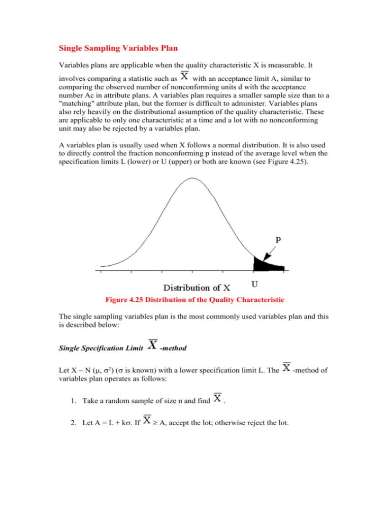
Single Sampling Variables Plan
Variables plans are applicable when the quality characteristic X is measurable. It
involves comparing a statistic such as
with an acceptance limit A, similar to
comparing the observed number of nonconforming units d with the acceptance
number Ac in attribute plans. A variables plan requires a smaller sample size than to a
"matching" attribute plan, but the former is difficult to administer. Variables plans
also rely heavily on the distributional assumption of the quality characteristic. These
are applicable to only one characteristic at a time and a lot with no nonconforming
unit may also be rejected by a variables plan.
A variables plan is usually used when X follows a normal distribution. It is also used
to directly control the fraction nonconforming p instead of the average level when the
specification limits L (lower) or U (upper) or both are known (see Figure 4.25).
Figure 4.25 Distribution of the Quality Characteristic
The single sampling variables plan is the most commonly used variables plan and this
is described below:
Single Specification Limit
-method
Let X ~ N (, ) ( is known) with a lower specification limit L. The
variables plan operates as follows:
1. Take a random sample of size n and find
2. Let A = L + k. If
.
 A, accept the lot; otherwise reject the lot.
-method of
In the case of an upper specification limit, A is set as U-k and the acceptance
criterion is reversed as
k (or A).
 A (see Figure 4.26). The parameters of the plan are n and
Figure 4.26 Operation of Xbar Method
k-method
When  is unknown, it is estimated by the sample standard deviation S (n-1 in
divisor) and the plan operates as follows:
1. Draw a random sample of size n and compute Z = ( - L) / S
2. If Z  k, accept the lot; otherwise, reject the lot. Equivalently, accept the lot
when
- kS  L
In the case of an upper specification limit, Z is computed as
Z = (U -
)/S
and the acceptance criterion remains the same as Z  k (or
+ kS  U). The
parameters of the plan are n and k. The operation of the k-method plan is shown in
Figure 4.27. It is also noted that the
and k methods are equivalent if  is known.
Figure 4.27 Operation of k-Method Plan
For given AQL (p1), LQL (p2), producer's risk () and consumer's risk ( ), the
formulae for n and k are:
k=
where Z is the standard normal deviate with (upper) tail area  .
For example, if AQL = 1%,  = 5%, LQL = 4% and  = 5%, the variables plan
parameters are found as
k=
= 2.04
n=
= 32.7  33 ( known)
= 32.7 (1 +
)= 100.7  101 ( unknown).
Note that the matching single sampling attribute plan requires a sample of size 296 for
the same conditions.
The formula for n when  is unknown is based on the normal approximation and is
found to work well even though (U -
) / s follows a noncentral t distribution.
M-method
The operating procedure of the variables plan is also modified using the uniform
minimum variance unbiased estimate of the lot fraction nonconforming p. In case of a
lower specification limit, the quantity
is the minimum variance unbiased estimate of p. The estimate
is compared
with the maximum allowable proportion of nonconforming M and the lot is accepted
if
 M. This procedure is known as the M-method of operation of the variables
plan. Note that k is defined using QL by the relation:
In case of an upper specification limit, the standard normal deviate
or
is used and the acceptance criterion remains the same. The M-method is also
equivalent to the k-method of operation of the plan.
The OC curve of the single sampling variables plan is drawn using the relationships
(k - Zp)
= Z1-Pa (known)
 unknown)
The following graphs (Figure 4.28) show the relationships between the auxiliary
variables Zp and Z1-Pa.
Figure :Relationship Between p and Pa
The formulae for the AOQ and ATI functions remain the same as that of a single
sampling attributes plan with Pa found from the above relationship. To draw the OC
curve, usually a value for Pa is assumed and p is then obtained. Appendix A4.10
shows how to run MINITAB local macros for designing a variables plan and drawing
its OC, AOQ and ATI curves.
Double specification limits are beyond the scope of this course. However, they are
necessary when the limits are fairly tight in relation to the inherent product variability.
Otherwise, single specification limit plans may be used.
In the case of a double specification limit, the proportion nonconforming may be a
result of products lying beyond both the upper and lower specification limits at the
same time if the variability is large. Two single specification limits can be used if the
specification limits are very wide so that the occurrence of a product outside either of
the limits is mutually exclusive. If
Zpm =
then pm is the minimum proportion nonconforming outside one
of the specification limits. If pm is large, it means that the limits may be unrealistically
narrow. For example, if 2pm > LQL, it means that a batch is always unacceptable and
must be rejected. If 2pm > AQL, it means that a batch can never be acceptable. This
suggests that the specification limits are too tight and should be loosened (widened)
slightly. If
< 2pm < AQL, the specification limits are still too narrow but
one may proceed if a double specification limit variables plan is used. This type of
plan is however beyond the scope of this course. Only if 2pm <
may a single
specification limit plan be used because the specification units are attainable for this
product variability level(s).
To select a variables scheme for given lot size and AQL, MIL-STD-414 tables were
used. The switching rules of MIL-STD-414 were based on the estimation of the
process average, unlike its attribute counterpart MIL-STD-105 E. These rules have
been modified in the ISO standard ISO 3951:1989(E), Sampling Procedures and
Charts for Inspection by Variables for Percent Nonconforming. For an example for
the application of variables plans, one may refer to ISO 8197:1988(E) Milk and Milk
Products - Sampling Inspection by Variables. This standard lists variable plans for
normal, reduced and tightened inspections indexed by AQL and lot size. For an AQL
of 1%, the following normal plans are listed in the standard:
Lot Size
up to 50
51 to 90
91 to 150
151 to 280
281 to 500
501 to 1200
1201 to 3200
3201 to 10,000
10,001 to 35,000
35,001 to 150,000
150,001 to 500,000
500,001 & above
n
4
5
7
10
15
20
25
35
50
75
100
150
k
1.45
1.53
1.62
1.72
1.79
1.82
1.85
1.89
1.93
1.98
2.00
2.03