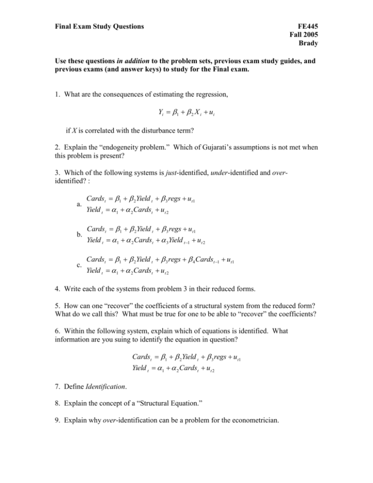
Final Exam Study Questions
FE445
Fall 2005
Brady
Use these questions in addition to the problem sets, previous exam study guides, and
previous exams (and answer keys) to study for the Final exam.
1. What are the consequences of estimating the regression,
Yi  1   2 X i  ui
if X is correlated with the disturbance term?
2. Explain the “endogeneity problem.” Which of Gujarati’s assumptions is not met when
this problem is present?
3. Which of the following systems is just-identified, under-identified and overidentified? :
a.
b.
c.
Cardst  1   2Yield t   3 regs  u t1
Yield t   1   2 Cardst  u t 2
Cardst  1   2Yield t   3 regs  u t1
Yield t   1   2 Cardst   3Yield t 1  u t 2
Cardst  1   2Yield t   3 regs   4 Cardst 1  u t1
Yield t   1   2 Cardst  u t 2
4. Write each of the systems from problem 3 in their reduced forms.
5. How can one “recover” the coefficients of a structural system from the reduced form?
What do we call this? What must be true for one to be able to “recover” the coefficients?
6. Within the following system, explain which of equations is identified. What
information are you suing to identify the equation in question?
Cardst  1   2Yield t   3 regs  u t1
Yield t   1   2 Cardst  u t 2
7. Define Identification.
8. Explain the concept of a “Structural Equation.”
9. Explain why over-identification can be a problem for the econometrician.
Final Exam Study Questions
FE445
Fall 2005
Brady
10. Explain the concept of Instrumental Variables.
11. Define “Two Stage Least Squares.”
12. Consider the following system:
Cardst  1   2Yield t   3 regs   4 Cardst 1  u t1
Yield t   1   2 Cardst  u t 2
a. Which of these equations can you identify?
b. Which variable do need to “instrument” for? Which variables can be used as
instruments?
c. Write this system in its reduced form.
d. Explain how to estimate an instrument from the reduced form equations.
e. Using the reduced form equation, write the equation for the Instrument:
IV = ?.
f. Why is this procedure preferable to simply picking your own instrument out
of those available in the system?
g. What are the two “stages” of 2SLS?
Panel Data
Describe the advantages of estimating with panel data.
Assume we have 20 years of data on four firms. Assume you “pool” the data and
estimate the regression,
Yit  1   2 X it   3 X 2it   4 X 3it  uit
Explain the problems that would arise if you went ahead and estimated this model
assuming that the coefficients were constant across time and individuals.
Define the Fixed Effects Model. What assumptions are made to estimate this model?
Describe how you estimate the Fixed Effects model in practice. Write the model you
would estimate.
Explain the alternative assumptions you can place on the Fixed Effects model.
Explain how you would go about estimating the Fixed Effects model when all
coefficients vary across individuals. Write the model you would estimate.
Final Exam Study Questions
FE445
Fall 2005
Brady
List and describe four general problems you might encounter in using the Fixed Effects
Model.
Cite four possible modifications you can make to the classical assumption (that may be
necessary) when estimating the Fixed Effects model.
Distributed Lag and Autoregressive Models
Write an econometric model that includes both autoregressive terms and distributed lag
terms (as explanatory variables).
Consider the model: Yt  1   2 X t   3 X t 1   4 X t 2  uit .
What is the short run multiplier in this model?
What is the long run multiplier in this model?
Describe some reasons for including distributed lags as explanatory variables (why might
it be appropriate to include the terms as regressors?).
Define and explain the Koyck distribution.
Explain the Koyck transformation. Why do we need to do such a transformation in the
first place?
If  k   0 k where k  0,1,... , explain it makes economic sense to assume that   1
(that is, why does it make sense to assume that the betas decline geometrically with
time?).
Describe Adaptive Expectations. What is advantage of this model over the partial
adjustment model?
Qualitative Response Models
Explain the usefulness of estimating a Qualitative Response Model.
Explain why the conditional probability of Yi in the LPM model is equal to pi. (Hint:
show what the expected value of a variable that follows the Bernoulli distribution).
List and describe the four main problems with the LPM.
Explain the intuition why the Goodness of Fit measure (R2) is inappropriate in the LPM
model (inadequate for capturing the dichotomous nature of a qualitative dependent
variable).
Why does the Cumulative Distribution Function make more sense for characterizing a
qualitative dependent variable? Why is the Logit Model (and the assumption of the CDF
distribution) an improvement over the LPM model?