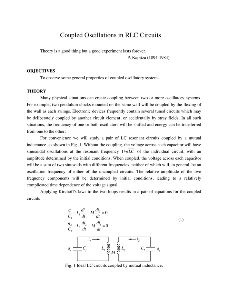
Coupled Oscillations in RLC Circuits
Theory is a good thing but a good experiment lasts forever.
P. Kapitza (1894-1984)
OBJECTIVES
To observe some general properties of coupled oscillatory systems.
THEORY
Many physical situations can create coupling between two or more oscillatory systems.
For example, two pendulum clocks mounted on the same wall will be coupled by the flexing of
the wall as each swings. Electronic devices frequently contain several tuned circuits which may
be deliberately coupled by another circuit element, or accidentally by stray fields. In all such
situations, the frequency of one or both oscillators will be shifted and energy can be transferred
from one to the other.
For convenience we will study a pair of LC resonant circuits coupled by a mutual
inductance, as shown in Fig. 1. Without the coupling, the voltage across each capacitor will have
sinusoidal oscillations at the resonant frequency 1/ LC of the individual circuit, with an
amplitude determined by the initial conditions. When coupled, the voltage across each capacitor
will be a sum of two sinusoids with different frequencies, neither of which will, in general, be an
oscillation frequency of either of the uncoupled circuits. The relative amplitude of the two
frequency components will be determined by initial conditions, leading to a relatively
complicated time dependence of the voltage signal.
Applying Kirchoff's laws to the two loops results in a pair of equations for the coupled
circuits
di
di
q1
− L1 1 − M 2 = 0
C1
dt
dt
q2
di
di
− L2 2 − M 1 = 0
C1
dt
dt
(1)
i2
i1
q
1
C1
L1
M
L2
C2
q
2
Fig. 1 Ideal LC circuits coupled by mutual inductance.
We then use the fact that
i1 = −
dq1
dt
i2 = −
dq2
dt
(2)
and define some convenient parameters
ω102 = 1/L1C1
m1 = M /L1
2
ω 20
= 1/L2C2
m2 = M /L2
(3)
to obtain the coupled second order equations
d 2q1
d 2q2
+ m1 2 + ω102q1 = 0
2
dt
dt
2
d q2
d 2q1
2
+
m
+ ω 20
q2 = 0
2
dt 2
dt 2
(4)
We assume a solution of the form
q1 = A1 e iωt
q2 = A2 e iωt
(5)
and substitute to get two algebraic equations in ω and A1, A2
ω 2 A1 + ω 2 m1 A2 − ω102 A1 = 0
2
ω 2 A2 + ω 2 m2 A1 − ω 20
A2 = 0
(6)
The equations have solutions provided that ω is chosen to be
2
2
2 1/ 2
(ω102 + ω 20
) ± [(ω102 + ω 20
) − 4(1− m1m2 )ω102ω 20
]
ω =
2(1− m1m2 )
2
±
(7)
and that A1, A2 are related by
ω102 − ω 2
A2 =
A1
ω 2 m1
Physics 231 Coupled Oscillations
(8)
2
The general solutions for q1, q2 are superpositions of terms corresponding to each of the allowed
frequencies
q1 = B1 e iω + t + B2 e−iω + t + B3 e iω − t + B4 e−iω − t
(9)
and a similar expression for q2 with coefficients that satisfy Eq. 8. To get a solution in terms of
real cosine functions, let
B1 = 12 D1e iφ1
B2 = 12 D1e−iφ1
B3 = 12 D2e iφ 2
B4 = 12 D2e−iφ 2
(10)
ω102 − ω +2
ω102 − ω−2
cos(
ω
t
+
φ
)
+
D
cos(ω− t + φ 2 )
+
1
2
ω +2 m1
ω−2 m1
(11)
Substituting into Eq. 9, we finally get
q1 = D1 cos(ω + t + φ1 ) + D2 cos(ω− t + φ 2 )
q2 = D1
This shows that both q1 and q2 are superpositions of two sine waves with amplitude and phase
determined by the initial conditions.
Some simplification is possible if we consider the important special case of identical
oscillators, so that ω10 = ω20 = ω0 and m1 = m2 = m. Then
ω +2 =
ω 02
1− m
ω−2 =
ω 02
1+ m
(12)
which shows that the new oscillation frequencies are both shifted from ω0. For initial conditions
such that capacitor C1 is fully charged, C2 has no charge, and the currents are zero, we find that
D1 = D2 and φ1 = φ2. The resulting equal-amplitude sine waves will show a clear beat pattern at
the difference frequency, and the beats on q1 and q2 will be phase shifted by π. It will be easy to
test this prediction experimentally by observing the time dependence of q1 and q2.
When the oscillators are not identical, oscillations will still occur at two distinct
frequencies, but the amplitudes will not necessarily be equal, and beats may not be evident.
These effects can be seen qualitatively in the time dependence but a mode plot, shown in Fig. 2,
is a simpler way to verify the calculation. This is a plot of ω+ and ω- vs ω10 when ω20 is fixed,
which shows how the coupled frequencies vary with the difference between the uncoupled
frequencies. Note the odd fact that ω+ and ω- never become equal, a phenomenon called an
avoided crossing which is characteristic of coupled linear systems.
Physics 231 Coupled Oscillations
3
1.8
normalized mode frequencies
1.6
1.4
1.2
1.0
0.8
0.6
0.4
0.2
0.2
0.4
0.6
0.8
ω
1.0
10
/ω
1.2
1.4
1.6
1.8
20
Fig. 2 Mode plot for coupled oscillators. The dashed lines represent the uncoupled frequencies,
while the solid lines are ω+ and ω- for the coupled system. All frequencies are scaled to ω20.
EXPERIMENTAL PROCEDURE
The time dependence of the coupled oscillations will be examined by plotting the
voltages across C1 and C2 as a function of time during free oscillation. The mode plot will be
constructed by driving one of the oscillators and looking for the frequencies that give maximum
voltage across C1 or C2. The two methods require slightly different circuits and will be discussed
separately.
1. Free oscillation
Set up the circuit as shown in Fig. 3, using the large solenoids as L1 and L2. The solenoids
should be aligned coaxially and as close together as possible to maximize coupling. Capacitor C1
is the 0.1 µF capacitor from the capacitor column on the patch board, and C2 is the 0.1 µF
capacitor near the 3.3Ω resistor. Connections to the LabQuest interface should be made as
shown, and the LoggerPro software started from Coupled.cmbl to configure the data acquisition.
To measure the time dependence, set the switch to charge the capacitor, click on Collect
and then flip the switch. If the mechanical switch contacts bounce you may see some anomalies
Physics 231 Coupled Oscillations
4
Power
Supply
+
LabQuest
chan 1 + chan 2 +
b
a
L2
L1
C1
chan 1 -
C2
chan 2 -
Fig. 3 Circuit for observing time dependence of q1 and q2. The power supply must be set to 10V
to insure proper triggering of the LabQuest interface.
at the start of the traces. Repeat the acquisition procedure until you get clear oscillations on both
channels. The software will display the time dependence of both voltages and the frequency
spectrum of the oscillations.
According to the discussion above, the oscillations in this case should be described as the
sum of two sine waves at slightly different frequencies, with damping due to the finite resistance
in the circuit. The oscillation frequencies of V1 and V2 should be the same, as shown by the peaks
in the respective FFT (fast Fourier transform) plots. To test this assertion more quantitatively, fit
the data for V1 to the appropriate function from the Curve Fit menu. Is this an adequate description
of the time dependence? What happens if you repeat the measurement with weaker coupling,
achieved by moving the solenoids a few centimeters apart? How is this explained by Eq. 12?
To examine the response of nonidentical oscillators, push the solenoids together to get
maximum coupling and change C1 to get a different ω1. Using the FFT plots, compare the
relative amplitudes of ω+ and ω- between the V1 and V2 signals for two or three ω1. Do you
recognize any pattern of the relative amplitudes as you change ω1?
2. Driven oscillations
Figure 4 shows the circuit for measuring the mode curve by determining the peak
response frequencies. Sine-wave excitation is provided by the function generator, with the
oscilloscope used as a voltmeter. If you slowly sweep the function generator through the
frequency range around the resonances you will notice two relative maxima in V1 and V2,
corresponding to ω+ and ω-. (The function generator reads frequency, not angular frequency, so it
is easier to work with f+ and f- for this section.)
Arrange the solenoids for maximum coupling and find f+ and f- using the available
capacitor values on the board for C1 while keeping C2 at 0.1 µF. You also need to measure f1 for
Physics 231 Coupled Oscillations
5
Oscilloscope
Chan 2
Chan1
Red
Red
red
3.3 Ω
black
L2
L1
C1
Chan 1
Black
C2
Chan 2
Black
Fig. 4 Circuit for driving coupled LC circuits. Note the 3.3Ω resistor which decreases the
effective output resistance of the function generator to minimize damping. External triggering
from the TTL output of the function generator will give the most stable display and an accurate
readout of the frequency on the scope screen.
each C1 capacitor value when the solenoids are separated sufficiently that the coupling is
negligible. Use these data to construct a mode plot. Does the result look like Fig. 2? Are the
frequencies for the f1 = f2 case the same as those found by fitting the time dependence?
If you are familiar with Matlab you can use the file mode_plot.m available on the PHYS
231 web page to plot your data and compare it to Eq. 7. In addition to the data above, you will
also need f2 in the uncoupled case, to characterize that oscillator. The parameter m can be
adjusted for best fit.
REPORT
Your report should include your fits of the time dependence data, the mode plot, and a
discussion of your results.
Physics 231 Coupled Oscillations
6