Elementary Forecasting Methods
A Time Series is a set of regular observations Zt taken over time. By the term spot estimate
we mean a forecast in a model that works under deterministic laws.
Exponential Smoothing.
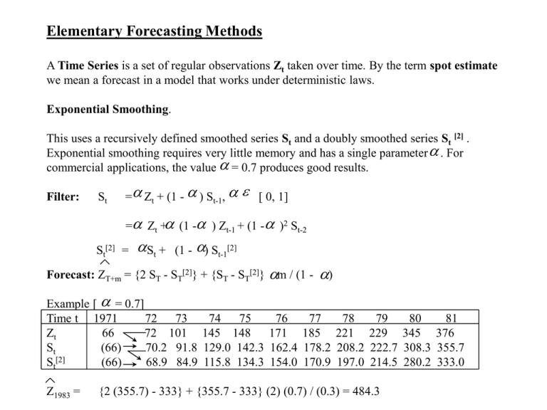
This uses a recursively defined smoothed series St and a doubly smoothed series St [2] .
Exponential smoothing requires very little memory and has a single parameter  . For
commercial applications, the value  = 0.7 produces good results.
Filter:
St
= Zt + (1 -  ) St-1, 
 [ 0, 1]
= Zt + (1 - ) Zt-1 + (1 - )2 St-2
St[2] =
 St +
(1 -
) St-1[2]
Forecast: ZT+m = {2 ST - ST[2]} + {ST - ST[2]} m / (1 Example [  = 0.7]
Time t 1971
72
73
Zt
66
72 101
St
(66)
70.2 91.8
St[2]
(66)
68.9 84.9
Z1983 =
74 75
145 148
129.0 142.3
115.8 134.3
76
171
162.4
154.0
)
77
185
178.2
170.9
78
221
208.2
197.0
79
229
222.7
214.5
{2 (355.7) - 333} + {355.7 - 333} (2) (0.7) / (0.3) = 484.3
80
81
345 376
308.3 355.7
280.2 333.0
Moving Average Model.
If the time series contains a seasonal component over n “seasons”, the Moving Average
model can be used to generate deseasonalised forecasts.
t  n 1
Filter:
Mt
= 
i t
Xi / n = Mt - 1 + { Zt - Zt - n } / n
t  n 1
Mt[2]
= 
Mt / n
i t
Forecast: ZT + k= { 2 (MT - MT[2]) } + { MT - MT[2] } 2 k / ( n - 1)
Example.
Time t 1988
1989
Sp Su Au Wi Sp Su Au
ZT
5 8
5 13
7 10
6
MT
- 7.75 8.25 8.75 9.00
MT[2]
- - 8.44
1990
1991
Wi Sp Su Au Wi Sp Su Au Wi
15 10 13 11 17 12 15 14 20
9.50 10.25 11.00 12.25 12.75 13.25 13.75 14.50 15.25
8.88 9.38 9.94 10.75 11.56 12.31 13.00 13.56 14.19
The deseasonalised forecast for Sp 1992, which is 4 periods beyond the last observation, is
ZT+4 = { 2 (15.25 - 14.19) } + { 15.25 - 14.19 } 2 (4) / 3 = 19.14
In simple multiplicative models we assume that the components are
Zt = T (trend) * S(seasonal factor) * R (residual term).
The following example demonstrates how to extricate these components from a series.
Time
t
Sp 1988
(1) Raw
(2) Four Month (3) Centered (4) Moving (5) Detrended (6) Deseasonalised (7) Residual
Data
Moving Total Moving Total Average
Data (1) / (4) Data (1)/(Seasonal) Series (6) / (4)
Zt =T*S*R
T*R
T
T
S*R
T*R
R
5
--
--
--
5.957
--
--
--
--
7.633
--
64
8.000
62.500
7.190
89.875
68
8.500
152.941
9.214
108.400
71
8.875
78.873
8.340
93.972
74
9.250
108.108
9.541
103.146
79
9.875
60.759
8.628
87.363
85
10.625
141.176
10.631
100.057
93
11.625
86.022
11.914
102.486
100
12.500
104.000
12.403
99.224
104
13.000
84.615
15.819
121.685
108
13.500
125.926
12.049
89.252
113
14.125
84.956
14.297
101.218
119
14.875
100.840
14.311
96.208
--
Su
8
31
Au
5
33
Wi
13
35
Sp 1989
7
Su
10
Au
6
36
38
41
Wi
15
44
Sp 1990
10
49
Su
13
Au
11
Wi
17
51
53
55
Sp 1991
12
58
Su
15
61
Au
14
Wi
20
---
---
---
20.133
--
---
---
---
14.175
--
--
The seasonal data is got by rearranging
column (5). The seasonal factors are then
reused in column (6)
Sp
1988
-1989 78.873
1990 86.022
Due to round-off errors in the arithmetic,
1991 84.956
it is necessary to readjust the means, so
Means 83.284
that they add up to 400 (instead of 396.905). Factors 83.933
The diagram illustrates the components
present in the data. In general when
analysing time series data, it is important
to remove these basic components before
proceeding with more detailed analysis.
Otherwise, these major components will
dwarf the more subtle component, and
will result in false readings.
The reduced forecasts are multiplied by
the appropriate trend and seasonal
components, at the end of the analysis.
Su
-108.108
104.000
100.840
104.316
105.129
Au
62.500
60.759
84.615
-69.291
69.831
Wi
152.941
141.176
125.926
-140.014
141.106
Raw Data
20
Trend
10
1988
1989
1990
1991
The forecasts that result from the models above, are referred to as “spot estimates”. This is
meant to convey the fact that sampling theory is not used in the analysis and so no
confidence intervals are possible. Spot estimates are unreliable and should only be used to
forecast a few time periods beyond the last observation in the time series.
Normal Linear Regression Model
In the model with one independent variable, we assume that the true relationship is
y = b0 + b1 x
and that our observations (x1, y1), (x2, y2), … , (xn, yn) is a random sample from the bivariate
parent distribution, so that
y= 0+ 1x+ ,
where  -> N( 0, ).
If the sample statistics are calculated, as in the deterministic case, then  0,  1 and r are
unbiased estimates for the true values, b0, b1 and  , where r and  are the correlation
coefficients of the sample and parent distributions, respectively.
If
y=0+ 
1
x0 is the estimate for y given the value x0, then our estimate of  2 is
s2 = SSE / (n - 2) =  ( yi - yi )2 / (n - 2)
and
VAR [ y] = s2 { 1 + 1/n + (x0 - x ) 2 /  ( xi - x ) 2 }.
The standardised variable derived from y has a tn - 2 distribution, so confidence intervals for
the true value of y corresponding to x0 is
y0 + tn - 2 s
1 + 1/n + (x0 - x ) 2 /  ( xi - x ) 2 .
Example. Consider our previous regression example:
y = 23 / 7 + 24 / 35 x
xi
0
1
2
3
4
5
yi
3
5
4
5
6
7
yi
3.286 3.971 4.657 5.343 6.029 6.714
2
(yi - yi ) 0.082 1.059 0.432 0.118 0.001 0.082
=>
 ( yi - yi )2 = 1.774, s2 = 0.4435,
 (x - x )2 = 17,5,
x = 2.5,
i
Let
Then
f(x0) = t4, 0.9 s 1 + 1/n + (x0 - x )2 /
x0
0
1
2
3
f(x0)
2.282 2.104 2.009 2.009
y0 - f(x0) 1.004 1.867 2.648 3.334
y0 + f(x0) 5.568 6.075 6.666 7.352
The diagram shows the danger of extrapolation.
It is important in forecasting that the trend is
initially removed from the data so that the
slope of the regression line is kept as close to
zero as possible.
A description of the Box-Jenkins methodology
and Spectral Analysis, which are the preferred
techniques for forecasting commercial data, is
to be found in standard text books.
(6)
7.40
s
= 0.666,
t4, 0.95 = 2.776, t4, 0.95 (s) = 1.849
 (xi - x )2 .
95% Confidence
4
2.104
3.925
8.133
Interval when x=6
5
6
2.282 2.526
4.432 4.874
8.996 9.926
8
Y
6
4
2
X
6