Example 2.2.6 Stiff Ordinary Differential Equations
> restart:
> with(plots):
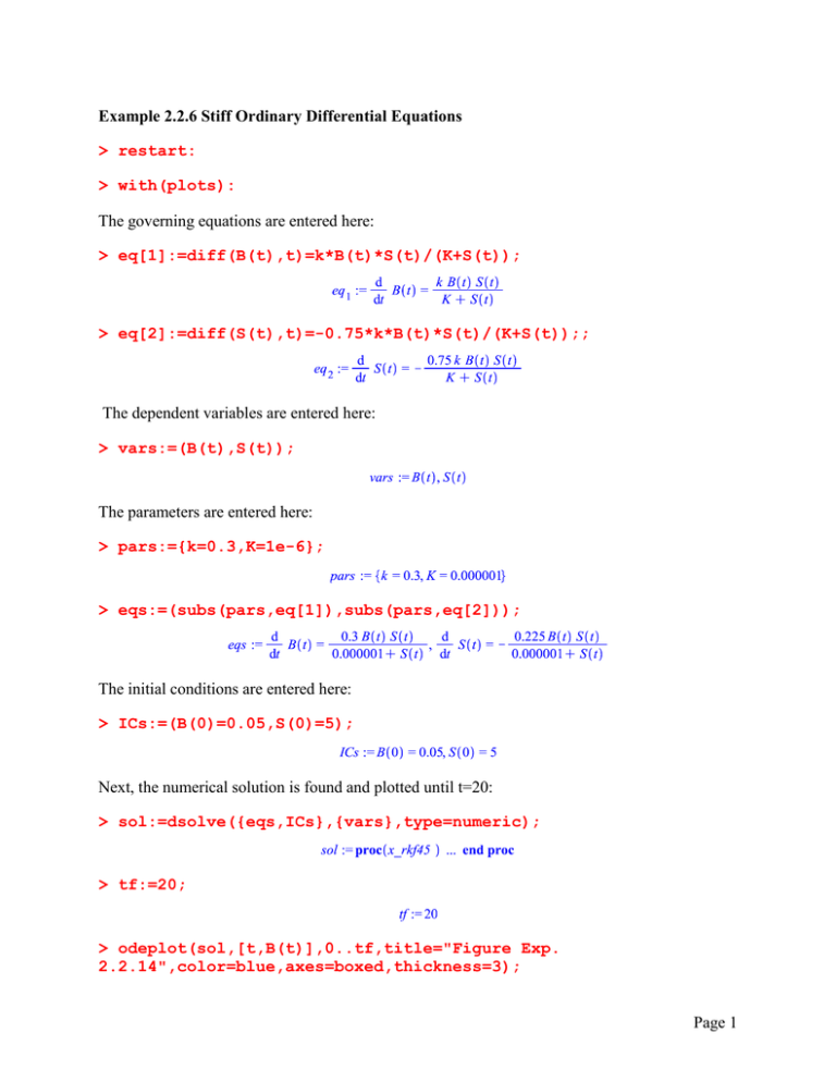
The governing equations are entered here:
> eq[1]:=diff(B(t),t)=k*B(t)*S(t)/(K+S(t));
> eq[2]:=diff(S(t),t)=-0.75*k*B(t)*S(t)/(K+S(t));;
The dependent variables are entered here:
> vars:=(B(t),S(t));
The parameters are entered here:
> pars:={k=0.3,K=1e-6};
> eqs:=(subs(pars,eq[1]),subs(pars,eq[2]));
The initial conditions are entered here:
> ICs:=(B(0)=0.05,S(0)=5);
Next, the numerical solution is found and plotted until t=20:
> sol:=dsolve({eqs,ICs},{vars},type=numeric);
> tf:=20;
> odeplot(sol,[t,B(t)],0..tf,title="Figure Exp.
2.2.14",color=blue,axes=boxed,thickness=3);
Page 1
> odeplot(sol,[t,S(t)],0..tf,title="Figure Exp.
2.2.15",color=blue,axes=boxed,thickness=3);
We observe that Maple predicts negative concentration. This is because the default absolute
error in 'dsolve' numeric is only 1d-6, which can be decreased to predict more accurate solutions:
> sol:=dsolve({eqs,ICs},{vars},type=numeric,abserr=1e-10);
Page 2
> odeplot(sol,[t,B(t)],0..tf,title="Figure Exp.
2.2.16",axes=boxed,thickness=3);
Warning, cannot evaluate the solution further right of 16.734694, maxfun
limit exceeded (see ?dsolve,maxfun for details)
> odeplot(sol,[t,S(t)],0..tf,title="Figure Exp.
2.2.17",axes=boxed,thickness=3);
Warning, cannot evaluate the solution further right of 16.734694, maxfun
limit exceeded (see ?dsolve,maxfun for details)
Maple's default Runge-Kutta method cannot predict the profiles after T=16.3. In addition, the
Page 3
program takes too long to run. This is a still problem and can be conveniently solved by using
Maple's still solver.
>
sol:=dsolve({eqs,ICs},{vars},type=numeric,stiff=true,abserr=1e10);
> odeplot(sol,[t,B(t)],0..tf,title="Figure Exp. 2.2.18",
color=green,axes=boxed,thickness=3);
> odeplot(sol,[t,S(t)],0..tf,title="Figure Exp.
2.2.19",color=green,axes=boxed,thickness=3);
>
Page 4
>
Page 5