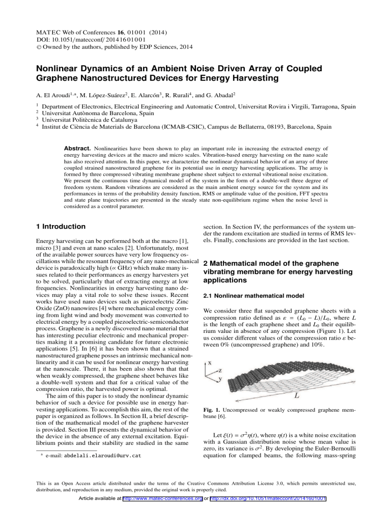
MAT EC Web of Conferences 16, 010 01 (2014)
DOI: 10.1051/matecconf/ 201 4 16 010 01
C Owned by the authors, published by EDP Sciences, 2014
Nonlinear Dynamics of an Ambient Noise Driven Array of Coupled
Graphene Nanostructured Devices for Energy Harvesting
A. El Aroudi1,a , M. López-Suárez2 , E. Alarcón3 , R. Rurali4 , and G. Abadal2
1
2
3
4
Department of Electronics, Electrical Engineering and Automatic Control, Universitat Rovira i Virgili, Tarragona, Spain
Universitat Autònoma de Barcelona, Spain
Universitat Politècnica de Catalunya
Institut de Ciència de Materials de Barcelona (ICMAB-CSIC), Campus de Bellaterra, 08193, Barcelona, Spain
Abstract. Nonlinearities have been shown to play an important role in increasing the extracted energy of
energy harvesting devices at the macro and micro scales. Vibration-based energy harvesting on the nano scale
has also received attention. In this paper, we characterize the nonlinear dynamical behavior of an array of three
coupled strained nanostructured graphene for its potential use in energy harvesting applications. The array is
formed by three compressed vibrating membrane graphene sheet subject to external vibrational noise excitation.
We present the continuous time dynamical model of the system in the form of a double-well three degree of
freedom system. Random vibrations are considered as the main ambient energy source for the system and its
performances in terms of the probability density function, RMS or amplitude value of the position, FFT spectra
and state plane trajectories are presented in the steady state non-equilibrium regime when the noise level is
considered as a control parameter.
1 Introduction
Energy harvesting can be performed both at the macro [1],
micro [3] and even at nano scales [2]. Unfortunately, most
of the available power sources have very low frequency oscillations while the resonant frequency of any nano-mechanical
device is paradoxically high (∝ GHz) which make many issues related to their performances as energy harvesters yet
to be solved, particularly that of extracting energy at low
frequencies. Nonlinearities in energy harvesting nano devices may play a vital role to solve these issues. Recent
works have used nano devices such as piezoelectric Zinc
Oxide (ZnO) nanowires [4] where mechanical energy coming from light wind and body movement was converted to
electrical energy by a coupled piezoelectric-semiconductor
process. Graphene is a newly discovered nano material that
has interesting peculiar electronic and mechanical properties making it a promising candidate for future electronic
applications [5]. In [6] it has been shown that a strained
nanostructured graphene posses an intrinsic mechanical nonlinearity and it can be used for nonlinear energy harvesting
at the nanoscale. There, it has been also shown that that
when weakly compressed, the graphene sheet behaves like
a double-well system and that for a critical value of the
compression ratio, the harvested power is optimal.
The aim of this paper is to study the nonlinear dynamic
behavior of such a device for possible use in energy harvesting applications. To accomplish this aim, the rest of the
paper is organized as follows. In Section II, a brief description of the mathematical model of the graphene harvester
is provided. Section III presents the dynamical behavior of
the device in the absence of any external excitation. Equilibrium points and their stability are studied in the same
a
e-mail: abdelali.elaroudi@urv.cat
section. In Section IV, the performances of the system under the random excitation are studied in terms of RMS levels. Finally, conclusions are provided in the last section.
2 Mathematical model of the graphene
vibrating membrane for energy harvesting
applications
2.1 Nonlinear mathematical model
We consider three flat suspended graphene sheets with a
compression ratio defined as ε = (L0 − L)/L0 , where L
is the length of each graphene sheet and L0 their equilibrium value in absence of any compression (Figure 1). Let
us consider different values of the compression ratio ε between 0% (uncompressed graphene) and 10%.
Fig. 1. Uncompressed or weakly compressed graphene membrane [6].
Let ξ(t) = σ2 η(t), where η(t) is a white noise excitation
with a Gaussian distribution noise whose mean value is
zero, its variance is σ2 . By developing the Euler-Bernoulli
equation for clamped beams, the following mass-spring
This is an Open Access article distributed under the terms of the Creative Commons Attribution License 3.0, which permits unrestricted use,
distribution, and reproduction in any medium, provided the original work is properly cited.
Article available at http://www.matec-conferences.org or http://dx.doi.org/10.1051/matecconf/20141601001
MATEC Web of Conferences
Table 1. Coefficients vi (i = 2, 4, 6, 8) for the potential energy for
different values of the compression ratio ε.
ε
0
0.025
0.05
0.075
0.1
v8 /56
6.57 · 1050
1.30 · 1051
2.56 · 1051
2.76 · 1051
3.89 · 1051
v6 /30
−5.73 · 1033
−1.36 · 1034
−2.29 · 1034
−2.34 · 1034
−3.43 · 1034
v4 /12
6.74 · 1016
9.26 · 1016
1.14 · 1017
1.16 · 1017
1.49 · 1017
ξ(t)
Vibration force
+
− −
−
1
m
Acceleration
1
s
Velocity
v1
1
s
v2 /2
0.0096
−0.036
−0.078
−0.112
−0.165
b
Damping factor
∂V
∂x
dynamic model is obtained for the considered coupled graphene
membranes [6]
∂V(x) ∂V(x) −
− b ẋ1 + σ2 η(t)(1)
m ẍ1 = −
∂x x=x1
∂x x=x2 −x1
∂V(x) ∂V(x) − b ẋ2 +
− b ẋ2 (2)
m ẍ2 = −
∂x x=x2 −x3
∂x x=x1 −x2
∂V(x) ∂V(x) m ẍ3 = −
− b ẋ3 +
− b ẋ2 (3)
∂x x=x3 −x4
∂x x=x2 −x3
∂V(x) ∂V(x) − b ẋ4 +
− b ẋ2 (4)
m ẍ4 = −
∂x x=x4
∂x x=x3 −x4
where xi , i = 1, 2, 3 are the displacements for the coupled
graphene membranes, m represents the effective mass of
each of the layers and b stands for their damping factor.
It should be noted that for simplicity it is assumed that all
the membranes are identic, i.e, they have the same mass
and the same damping coefficient. The potential energy is
given by [6]
1
1
1
1
v8 x8 + v6 x6 + v4 x4 + v2 x2
56
30
12
2
+
x 10
−19
1
V
E0
0
σ=0
0.025
0.05
0.075
0.1
E−
−1
−1.5
−1
E+
−0.5
0
x (nm)
0.5
1
−
−
1
s
1
m
v2
−
1
s
x2
b
∂V
∂x
−
−
+
1
s
1
m
Velocity
v3
−
1
s
x3
b
∂V
∂x
−
−
1
m
+
1
s
Velocity
v4
1
s
−
x4
b
Fig. 3. Simulink block diagram of four coupled graphene membranes.
(5)
The coefficients vi (i = 2, 4, 6, 8) are given in Table 1 for
different values of compression coefficient ε. These values
have been obtained by means of ab initio density-functional
calculations with the SIESTA code [6], [7] where the graphene
sheet is modeled at a fully atomistic level and its electronic
structure solved quantum mechanically. Figure 2 shows the
plot of V(x) in terms of the position x.
2
x1
Mass
∂V
∂x
V(x) =
Displacement
1.5
Fig. 2. Potential V(x) for different values of the compression factor ε. For ε 0, equilibrium points are also plotted. E+ and E−
are attractors while E0 is a saddle point. The
3 Dynamical behavior from numerical
simulations
3.1 Dynamics of a single graphene membrane
The nonlinear dynamics of a single graphene membrane
has been studied in [6] and [8]. We resume here the results
for comparison with the coupled graphene membranes. Let
also consider a compressed graphene with compression coefficient ε = 0.1 in such a way that the origin is a saddle point (non stable). The nonlinear model of the system
is numerically solved. A Matlab-simulink model was built
for the system equation modeling the graphene nano harvester device according to its mathematical model (Fig. 3).
A random excitation with a normal distribution and a maximum bandwidth ωbw is considered as a main input of the
system.
When such noise is applied to the system, the probability to swing between the two equilibrium point increases.
Consequently noise can be used to increase the RMS value
of the displacement and accordingly to raise the harvested
energy. Let us also consider a compressed graphene sheet
with compression coefficient ε 0 in such a way that the
origin is a saddle point (non stable). For some specific values of noise level, the system was simulated during 500 ns
and the time-series, phase space, probability density, and
amplitude spectra are plotted. Figures 4-5 show the dynamics of the system for different values of noise level.
The following particular cases are plotted in these figures
– σ2 = 1 pN, the noise intensity is weak and the system
evolves to the vicinity of one of the stable equilibrium
01001-p.2
350
400
450
500
200
−200
0
−300
−200
−400
250
400
350
Time (ns)
300
450
−400
−2
500
−1
0
Displacement x (nm)
Fig. 4. Dynamics of the graphene membrane under a random excitation σ2 = 1 pN (red), σ2 = 50.5 pN (green) and σ2 = 100 pN
(black).
30
40
Velocity v3 (m/s)
4
2
0
−2
−4
0
10
20
30
40
10
20
Time (ns)
30
40
10
20
30
40
10
20
Time (ns)
30
40
400
200
0
−200
10
20
Time (ns)
4
0
−2
−4
0
10
20
30
40
200
0
−200
−400
0
40
30
2
2
1
0
−1
−2
0
400
200
0
−200
−400
0
10
−210
−20
20
400
−200
0
10
−400
0
2
1
(b) Phase plane (x, v).
(a) Time series.
−2
0
400
Displacement x3 (nm)
Velocity v (m/s)
0
−100
Velocity v2 (m/s)
300
Velocity v1 (m/s)
−2
250
400
100
−1
Displacement x2 (nm)
200
−1
2
1
0
Displacement x4 (nm)
300
0
Velocity v4 (m/s)
400
1
Displacement x1 (nm)
2
Velocity (m/s)
Displacement x (nm)
CSNDD 2014
20
Time (ns)
30
200
0
−200
−400
0
40
−40
−230
−60
−240
N (dB)
−80
Fig. 6. Time domain waveforms of the displacements xi and velocities vi , (i = 1..4) corresponding to the four graphene membranes for two values of noise intensities.
−250
−260
−270
−100
−280
−120
−290
−1
0
Displacement x (nm)
1
2
−300 0
10
1
2
10
Frequency (GHz)
10
300
250
(a) Probability density func- (b) The FFT of x and σ η(t).
tion of x.
2
200
200
Velocity v1 (m/s)
150
Fig. 5. Spectrum and probability density function corresponding
to Fig. 4. Note that the spectrum is spread down to low frequency
regions when the noise intensity is sufficiently large so that the
potential barrier can be crossed.
3.2 Dynamics of the coupled membranes
In this section, only two values of noise intensity are considered, namely σ2 = 1 pN and σ2 = 50 pN, and different diagrams in the form of times series, state planes, FFT
spectra and probability density function of the displacement are obtained as for the single membrane case.
Figure 6 shows the time domain waveforms of the system. For low values of noise intensity the system stays
in the vicinity of the equilibrium point. For low values of
noise intensity the system stays in the vicinity of the equilibrium point.
50
0
−50
−100
−150
100
0
−100
−200
−200
−250
−1.5
Velocity v3 (m/s)
points X− or X+ depending on the initial conditions.
The probability to swing between the two equilibria is
almost zero. The vicinities of X− and X+ correspond to
the unique set with non-zero values of the probability
density function. The energy of the system is concentrated in a limited range of frequency near the resonant
frequency (≈ 50 GHz).
– σ2 = 50.5 pN, the noise intensity is sufficient to make
the system to leave the vicinity of the stable equilibrium points X− or X+ which makes the system to swing
between them. The range within which the displacement includes the interval (X− , X+ ). The equilibria X−
and X+ correspond to the maximum of the probability
density function.
– σ2 = 100 pN, the noise intensity is in such a way that
the probability of swinging between the stable equilibrium points X− or X+ is larger and the system presents
larger velocities and displacements and therefore the
harvested energy will also be larger.
100
Velocity v2 (m/s)
−140
−2
−1
−0.5
0
0.5
Displacement x1 (nm)
1
−300
−1.5
1.5
250
250
200
200
150
150
100
100
Velocity v4 (m/s)
Probability density (dB)
−220
50
0
−50
1
1.5
−2
−1
0
1
Displacement x4 (nm)
2
3
50
0
−100
−150
−150
−250
−3
−0.5
0
0.5
Displacement x2 (nm)
−50
−100
−200
−1
−200
−2
−1
0
1
Displacement x3 (nm)
2
3
−250
−3
Fig. 7. The state space in the planes (xi , vi ), (i = 1..4) corresponding to the four graphene membranes for two values of noise intensities.
Figure 7 shows the projection of the state plane time of
the system in the planes (xi , vi ), (i = 1..4) corresponding
to each graphene membrane. For relatively high values of
noise intensity, the trajectory can only evolve to an equilibrium point being the ambient vibration in this case not
sufficient to make the system to oscillate between the two
regions. When the noise intensity increases, as in the case
of the single membrane, the system trajectory visits more
the different equilibrium points and larger oscillation amplitude can be reached. All the four membranes are characterized by the same dynamics.
Figure 8 depicts the FFT spectra of the displacement
corresponding to each graphene membrane. While a clear
single resonant frequency can be observed for the low intensity noise case, the spectrum corresponding to a relatively high value of noise intensity is spread a broad range
of frequencies. This occurs for all the membranes.
Figure 9 shows the probability density functions calculated for the different displacements of the membranes.
For low values of noise intensity the probability of finding
the system in the vicinity of one of its equilibrium points is
01001-p.3
−200
−200
−220
−220
−240
−240
X2 (dB)
X1 (dB)
MATEC Web of Conferences
−260
−280
−300
−300
−1
0
10
10
Frequency (GHz)
−200
−200
−220
−220
−240
−240
−260
−280
−300
−300
−1
0
10
10
Frequency (GHz)
−1
10
Frequency (GHz)
This work was partially supported by the Ministerio de
Ciencia e Innovación under grant CSD2009-00046.
1
10
References
1.
−320
1
10
0
10
−260
−280
−320
Acknowledgments
−320
1
10
X4 (dB)
X3 (dB)
−260
−280
−320
when the noise level for a certain value of the compression
ratio.
−1
0
10
10
Frequency (GHz)
1
10
1
1
0.9
0.9
0.8
0.8
0.7
0.7
Probability density
Probability density
Fig. 8. FFT spectra of the displacements xi (i = 1..4) corresponding to the four graphene membranes for two values of noise intensities.
0.6
0.5
0.4
0.3
0.2
0.4
0.3
0.1
−1.5
−1
−0.5
0
0.5
Displacement x1 (nm)
1
1.5
0
−3
2
1
1
0.9
0.9
0.8
0.8
0.7
0.7
Probability density
Probability density
0.5
0.2
0.1
0
−2
0.6
0.6
0.5
0.4
0.3
0.2
−1
0
1
Displacement x2 (nm)
2
3
0.6
0.5
0.4
0.3
0.2
0.1
0
−2
−2
0.1
−1
0
1
Displacement x3 (nm)
2
3
0
−2
−1.5
−1
−0.5
0
0.5
Displacement x4 (nm)
1
1.5
2
Fig. 9. Probability density function of the displacements xi (i =
1..4) for two values of noise intensities. For reference, the probability density of the noise driving signal is also plotted
practically one. For relatively high values of noise intensity
the probability to visit a wider region increases being the
maximum probability that corresponding to the vicinity of
the equilibrium points.
L. Gammaitoni, H. Vocca, I. Neri, F. Travasso and
F. Orfei, “Vibration Energy Harvestng: Linear and
Nonlinear Oscillator Approaches," in Sustainable Energy Harvesting Technologies-Past, Present and Future, pp. 171-190, 2007.
2. Igor Neri, Flavio Travasso, Helios Vocca, Luca Gammaitoni, “Nonlinear noise harvesters for nanosensors,"
Nano Communication Networks vol. 2, no. 4, 2011,
pp. 230-234.
3. Huicong Liu; Cho Jui Tay; Chenggen Quan;
Kobayashi, T.; Chengkuo Lee; "Piezoelectric MEMS
Energy Harvester for Low-Frequency Vibrations With
Wideband Operation Range and Steadily Increased
Output Power," Journal of Microelectromechanical
Systems, vol.20, no.5, pp.1131-1142, Oct. 2011.
4. Sheng Xu, Yong Qin, Chen Xu, Yaguang Wei, Rusen
Yang and Zhong Lin Wang “Self-powered nanowire
devices," Nature nanotechnology, vol. 5, no. 5, 2010.
5. S. A. Imam, S. Sabri and T. Szkopek, "Low-frequency
noise and hysteresis in graphene field-effect transistors
on oxide S.A.," Micro and Nano Letters, IET, vol.5,
no.1, pp.37-41, Feb. 2010.
6. M. López-Suárez, R. Rurali, L. Gammaitoni and G.
Abadal “Nanostructured Graphene for Energy Harvesting," Physical Rweview B, vo. 84, No. 161401,
pp.1-5, 2011.
7. J. M. Soler, E. Artacho, J. D. Gale, A. García, J.
Junquera, P. Ordejon, and D. Sánchez-Portal, “The
SIESTA method for ab initio order-N materials simulation," J. Phys. Condens. Matter vol. 14, no. 11, pp.
2745, 2002.
8. A. El Aroudi, M. Lopez-Suarez, R. Rurali, E. Alarcon
and G. Abadal “Nonlinear Dynamics in a Nanostructured Graphene Device for Energy Harvesting Applications", IEEE International Symposium on Circuits
and Systems, 2013, ISCAS 2013, May 2013, pp. 27272730, Beijing, China.
Conclusions
In this paper we have considered the nonlinear dynamics of four identical coupled nanostructured graphene vibrating membranes for ambient energy applications at the
nanoscale. The compressed graphen present a nonlinearity
that has been shown to play an important role in increasing
the efficiency of this energy harvesting device by increasing the RMS values of the displacement and the velocity. We presented a continuous-time nonlinear dynamical
model of the coupled system. When random vibrations are
considered as the main ambient energy source for the system, the performances of the system as an energy harvester
are presented in the steady state non-equilibrium regime
01001-p.4