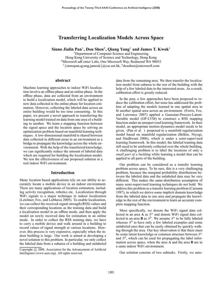
Proceedings of the Twenty-Third AAAI Conference on Artificial Intelligence (2008)
Transferring Localization Models Across Space
Sinno Jialin Pan1 , Dou Shen2 , Qiang Yang1 and James T. Kwok1
1
Department of Computer Science and Engineering
Hong Kong University of Science and Technology, Hong Kong
2
Microsoft adCenter Labs, One Microsoft Way, Redmond WA 98052
1
{sinnopan,qyang,jamesk}@cse.ust.hk, 2 doushen@microsoft.com
abstract
data from the remaining area. We then transfer the localization model from subarea to the rest of the building with the
help of a few labeled data in the interested areas. As a result,
calibration effort is greatly reduced.
Machine learning approaches to indoor WiFi localization involve an offline phase and an online phase. In the
offline phase, data are collected from an environment
to build a localization model, which will be applied to
new data collected in the online phase for location estimation. However, collecting the labeled data across an
entire building would be too time consuming. In this
paper, we present a novel approach to transferring the
learning model trained on data from one area of a building to another. We learn a mapping function between
the signal space and the location space by solving an
optimization problem based on manifold learning techniques. A low-dimensional manifold is shared between
data collected in different areas in an environment as a
bridge to propagate the knowledge across the whole environment. With the help of the transferred knowledge,
we can significantly reduce the amount of labeled data
which are required for building the localization model.
We test the effectiveness of our proposed solution in a
real indoor WiFi environment.
In the past, a few approaches have been proposed to reduce the calibration effort, but none has addressed the problem of adapting the models learned in one spatial area to
fit another spatial area across an environment. (Ferris, Fox,
and Lawrence 2007) applied a Gaussian-Process-LatentVariable model (GP-LVM) to construct a RSS mapping
function under an unsupervised learning framework. In their
model, an appropriate motion-dynamics model needs to be
given. (Pan et al. ) proposed to a manifold regularization
model based on manifold regularization (Belkin, Niyogi,
and Sindhwani 2006), which is under a semi-supervised
learning framework. In this model, the labeled training data
still need to be uniformly collected over the whole building.
A challenging problem is to label the locations of only a
small part of a building while learning a model that can be
applied to all parts of the building.
Our problem can be considered as a transfer learning
problem across space. To be sure, this is a very challenging
problem, because the marginal probability distributions between the labeled data and the unlabeled data may be very
different. This makes the same-distribution assumption of
many semi-supervised learning techniques do not hold. We
address this problem as a transfer learning problem (Caruana
1997), in which we derive some implicit domain knowledge
from the labeled data in one area and propagate the knowledge to the rest of the environment to learn an accurate complete mapping function.
Introduction
Many location based applications rely on our ability to accurately locate a mobile device in an indoor environment.
There are many applications of location estimation, including activity recognition, robotics etc. Localization through
WiFi signals is a major technique in indoor localization
(Letchner, Fox, and LaMarca 2005). To enable localization,
we can collect the received-signal-strength (RSS) values and
their corresponding locations as the training data and build
a localization model in an offline mode, and then apply the
model on newly received data for estimation in an online
mode. In order to collect the RSS training data, we have
to carry a mobile device and walk around in a building to
record values of signal strength at various locations. However, this process is very expensive, especially when the indoor building is large. Our work is aimed at developing a
novel solution to this problem. In particular, we only collect
the labeled data from a subarea of a building and unlabeled
More specifically, we denote the WiFi signal data collected in an area A as S a and denote WiFi signal data collected in an area B as S b . We assume S a to be fully labeled
whereas S b to have only a few labeled examples and some
unlabeled ones that can be easily obtained by quickly walking through the area. Our key observation is that there must
be some latent knowledge or common structure between S a
and S b , which can be used for propagating the label information across space, when the area A and the area B are in
a same indoor WiFi environment.
c 2008, Association for the Advancement of Artificial
Copyright Intelligence (www.aaai.org). All rights reserved.
Our solution consists of two subtasks. Firstly, we auto-
1383
matically extract the domain knowledge of an indoor environment from the labeled data collected in an area. We
formulate a quadratically constrained quadratic program
(QCQP) optimization problem (Boyd and Vandenberghe
2004) to solve this problem via a manifold of the WiFi signal
data. This manifold acts as a bridge that propagates the common knowledge across different areas. Secondly, we incorporate the extracted domain knowledge into a model to propagate the label information to unlabeled data collected in the
rest of the environment. We exploit the common knowledge
learned in the previous step as constraints and incorporate
them to another QCQP optimization problem to estimate labels of the unlabeled data collected in the rest of the environment. We empirically evaluate our proposed solution by
conducting experiments in a real office WiFi environment.
The experimental results show that our solution is quite effective in learning a high performance localization model
while reducing the calibration effort.
beled data to train the models. In order to reduce the calibration effort or the size of labeled data, (Ferris, Fox, and
Lawrence 2007) applied Gaussian-Process-Latent-Variable
models (GP-LVMs) to exploit the latent-space locations under an unsupervised framework. An assumption of this
model is that an accurate motion dynamics model is given,
which can benefit building a localization mapping function.
(Pan and Yang 2007) proposed to apply a semi-supervised
manifold technique for mobile device tracking in wireless
sensor networks. However, their model still needs to collect
labeled data through the whole indoor environment, which
cannot reduce the calibration effort dramatically. Our solution can derive implicit knowledge from the labeled data
collected in an area. By using the extracted knowledge, we
can reduce the labeled data collected in the rest of the building area dramatically while keeping the localization performance at a high level.
Transfer Learning for WiFi Localization
WiFi Localization in Indoor Environments
Problem Statement
Received-signal-strength (RSS) based indoor localization
and tracking methods have been increasingly popular for
WiFi networks (Bahl, Balachandran, and Padmanabhan
2000). The problem of RSS based indoor localization is to
estimate locations of a mobile device based on its RSS values. Consider a two-dimensional indoor localization problem. 1 A location is represented by ℓ = (x, y), where x and
y correspond to a value of x-coordinate and a value of ycoordinate, respectively. Assume that there are m transmitters, such as Access Points (APs), in an indoor environment,
which periodically send out wireless signals. A mobile device can receive signals sent by each of the m APs. Thus,
the signals received by a mobile device at a certain location
can be represented by a vector s = (s1 , s2 , ..., sm )T ∈ Rm .
The goal of a localization system is to estimate the location ℓi of a mobile device based the RSS vector si =
(si1 , si2 , ..., sim )T received by the mobile device. In an offline or training phase, a mapping function is learned from
a large amount of location-labeled RSS vectors collected at
various areas in a building. In an online phase, the learned
mapping function is used to locate the mobile device using
its real-time signal vectors. Here the locations of APs are
not necessarily known.
Consider a transfer learning problem for two-dimensional
WiFi indoor localization. Suppose that we have n1 signal
data collected in an area A. These data are denoted by S a
= {sai }, where sai = [sai1 , sai2 , . . . , saim ], i = 1, 2, . . . , n1 ,
and m is the number of APs. For simplicity, we assume
that all the n1 signal vectors in S a are labeled, which means
that the locations corresponding to all the signal vectors are
known2. In addition, we have n2 signal vectors collected in
the remaining area B of the indoor environment. These data
are denoted by S b ={sbi }, where sbi = [sbi1 , sbi2 , . . . , sbim ], and
i = 1, 2, . . . , n2 . We assume that the first l2 signal vectors
(where l2 ≪ n2 and l2 ≪ n1 ) in S b are labeled. Now, we
have two signal strength matrices Sna1 ×m and Snb 2 ×m , and
their label vectors La = [ℓa1 , ..., ℓan1 ] and Lb = [ℓb1 , ..., ℓbn2 ],
where ℓai is the labeled location of sai , for all i ≤ n1 . Similarly, ℓbi is the labeled location of sbi , if i ≤ l2 , otherwise, 03 .
Our goal is to automatically discover some shared knowledge (KB) in the indoor localization domain. Then we incorporate the KB and the data S a and S b to construct a
accurate mapping function for the whole environment, including both areas A and B.
Motivation
Existing approaches of RSS based localization fall into
two main categories: propagation-model based methods and
learning-based methods. Propagation-model based methods rely on indoor radio-signal propagation models. These
methods are poor in handling the uncertainty (Bahl, Balachandran, and Padmanabhan 2000). Learning-based methods apply machine learning techniques, such as Gaussian
processes (Ferris, Hähnel, and Fox 2006) and kernel methods (Nguyen, Jordan, and Sinopoli 2005), to handle the uncertainty in localization problems. A major drawback of
these methods is that they all require a large amount of la-
To achieve our goal of deriving implicit knowledge from the
training data collected in a certain subarea and then transferring it to the remaining area, we need to answer two questions. The first question is what knowledge can be extracted
from the signal strength data. As we know, once a wireless
communication system is set up in an indoor environment,
many APs are fixed at certain locations. Hence, unlike other
dynamic environmental factors such as the movement of furniture, these APs are often fixed at their original locations.
Intuitively, we can learn a more accurate mapping function
from the RSS values to locations once we have knowledge
1
The localization problem can be seen as a dimensionality reduction problem. Thus an extension to the three-dimensional case
is straight-forward.
2
3
1384
In general, some locations of S a can be unknown.
We use 0 to denote an unknown location.
of the APs’ locations, or at least their relative locations. We
can learn this important domain knowledge from the labeled
signal data collected in an area of the environment.
semi-supervised techniques to make the estimation more accurate (Ham, Lee, and Saul 2005). However, using only the
column data is not enough since the APs are usually far from
each other, which violates the basic assumption of manifold
methods. Furthermore, it is important to construct the mapping function simultaneously so that we can estimate the locations of the mobile devices at the same time. Fortunately,
recall the third domain characteristic mentioned in the previous subsection, namely that there should be certain relations
between the rows and the columns. This makes it possible to incorporate the similarities among the rows, the similarities among the columns and the similarities among the
rows and columns together to estimate the locations of APs
and building the mapping function. We call this process colocalization. In the following subsections, we first introduce
a preliminary implementation of co-localization in (Pan and
Yang 2007) and then present our important extension, which
addresses a major limitation of their model.
Our second question is how to make the best use of the
domain knowledge that we extract based on the labeled examples. As mentioned in the previous subsection, we have
two signal strength matrices S a and S b in hand. Let us
take S a as an example for explaining our idea. The signal
strength vector received by a mobile device in a certain location corresponds to an m-dimensional row in S a . In contrast, each AP is represented by a particular n1 -dimensional
column. Underlying the m-dimensional signal strength data
is a two-dimensional manifold, because these signal strength
data are collected by a mobile device moving around a twodimensional physical space. Likewise, underlying the n1 dimensional AP data is also a two-dimensional manifold, because all the APs are placed on a two-dimensional physical
floor4 . With the above observations, we come to three important domain characteristics implied by the signal strength
matrix: (1) If two rows in the signal strength matrix are similar to each other, it implies that the corresponding locations
where a mobile device receives the signals are close to each
other. (2) If two columns are similar to each other, it implies
that the locations of the two corresponding APs are close to
each other. (3) Each element saij reflects the signal strength
received by a mobile device at a certain location ℓ from the
jth AP. If the signal strength is strong, it implies that the
location ℓ is close to the location of the jth AP. Considering these characteristics, if the location information of the
APs is known, we can propagate the label information from
a data set S a to another data set S b , and then build a accurate
localization mapping function with S a and S b .
Initial Solution for Co-Localization The problem of colocalization described above can be solved through an the
optimization process outlined in the optimization problem
in (1) in an offline phrase. Note that our goal is to derive
knowledge of the APs’ locations from the labeled data collected in area A, thus the notations used in the optimization
problem in (1) are consistent with those related to S a given
in the Problem Statement section.
fx∗ =
arg
min
fx ∈R(n1 +m)
n1
X
n1 +l
|fxi − ℓxi |2 +
i=1
+γ1 fxT Lfx .
X
|fxi − ℓxi |2
i=n1 +1
(1)
where fx∗i is the estimated value of x-coordinate of a physical location corresponding to xi . Similarly, we can estimate
fy∗ by replacing x by y. Thus, f = [fx∗ , fy∗ ] ∈ R(n1 +m)×2 is
the location coordinate matrix of the mobile device and APs.
The first n1 rows of f are the location coordinates of the mobile device, and the last m rows are location coordinates of
APs. l is the number of labeled columns (corresponding to
APs whose locations are known), γ1 is a parameter to control the smoothness of coordinates along the manifold, and
L ∈ R(n1 +m)×(n1 +m) is the graph Laplacian matrix.
However, in reality, we cannot obtain the location information of all the APs in advance. For example, it is common
that an office building is taken by different companies and
these companies may set up their own APs. Due to privacy
reasons, people from one company may not know the positions of the APs set up by another company. Our transfer
learning approach for indoor localization aims at exploiting
data collected in a limited area to learn a mapping function
for the whole area. Therefore, we can first derive knowledge
of the APs’ location information from the abundant signal
data S a collected in area A. After that, we formalize the estimation of location labels of signal data S b (collected in an
area B) as an optimization problem and incorporate the derived knowledge as constraints. In this way, we can obtain
an accurate mapping function with S a , S b and their labels.
L should reflect three types of similarities: the similarities
between signal strength vectors si and sj (rows of S a ), the
similarities between APs and the similarities between APs
and signal strength vectors. For the first type of similarities,
we can use the rows of S a to compute the weight matrix
Ws = [wij ]n1 ×n1 , where wij = exp(−ksai − saj k2 /2σs2 ) if
sai is one of the k nearest neighbors of saj , or vice versa. The
corresponding graph Laplacian matrix is Ls = P
Ds − Ws ,
n
where Ds = diag(d1 , d2 , . . . , dn1 ) and di =
j=1 wij .
Similarly, we can construct the graph Laplacian matrix corresponding to the similarities between
APs:La = Da −Wa .
Ls 0
We expand Ls and La as L1 = 0
0
(n1 +m)×(n1 +m)
0 0
and L2 = 0 L
. The graph Lapla-
Discovering Domain Knowledge
We now discuss how to extract the location information of
the APs from the data S a collected in area A. In order to
estimate the locations (physical coordinates) of the APs, a
straightforward way is to apply manifold embedding techniques to the columns in S a , whose intrinsic dimensionality
is two. If some APs’ locations are known, we can apply
a
4
For simplicity, we do not consider the height of the APs since
the factor will not affect the localization performance.
(n1 +m)×(n1 +m)
cian matrix corresponding to the correlation between
1385
APs and
signal strength
vectors can be constructed as
D1
−S o
L3 = −S oT D
, where S o is the
2
because a similar derivation can be found in (Lanckriet et al.
2004)), the optimization problem in (3) can be rewritten as
the following QCQP problem:
(n1 +m)×(n1 +m)
original signal strength matrix, D1 and D2 are diagonal matrices which make the row sums zero (Hendrichson 2006).
Note that we use the Gaussian kernel to compute the weight
matrix and then construct L1 and L2 , while we use the original signal strength values in L3 . In order to make L3 comparable to L1 and L2 , we can transform S o = [soij ]n1 ×m
to a new matrix S ′ = [s′ij ]n1 ×m by the Gaussian kernel
2
s′ij = exp(−|soij − smax |2 /2σss
), where smax is the maximal signal strengthdetected by a mobile
device. Thus, L3 is
rewritten as L3 =
D1′
−S ′T
−S ′
D2′
min (fxi − ℓxi )T J(fxi − ℓxi ) + γ1 ct
fx ,t
subject to
, where D1′ and D2′ are
Encoding Domain Knowledge for Building Radio
Mapping
In the online phase, the corresponding location of a query
si = [si1 , si2 , . . . , sim ] is estimated using the method of
harmonic functions (Zhu, Ghahramani, and Lafferty 2003),
which is defined in Equation (2), as:
P
w f
Pj∈N ij j ,
j∈N wij
In the previous subsections, we have described what domain
knowledge can be extracted in the indoor localization problem and how to extract it automatically. In this subsection,
we present how to incorporate the extracted domain knowledge into the estimation of labels of the unlabel data collected in another area, and then construct the mapping function for the whole environment. Since the amount of labeled
data in S b is small, we cannot expect to obtain accurate location estimations of the unlabeled part in S b by solving the
optimization problem in (3) with S b or S a directly. However, since we have the extracted domain knowledge in terms
of the APs’ location information, we can reformulate the optimization problem in (3) so that we can take the knowledge
into consideration and consequently result in better location
estimation. The reformulated optimization problem is given
as follows:
(2)
where N is the set of k nearest neighbors of si in S a , wij
is the weight between si and saj which can be obtained as
described above, and fj is the location of saj solved from the
optimization problem in (1).
Extended Co-Localization The parameters µ1 , µ2 and µ3
for combining L1 , L2 , L3 are not easy to be tuned. We now
develop a method to automatically determine the parameters. In our method, we take the parameters as variables
and construct some constraints using these variables. By
imposing these constraints and reformulating the optimization problem in (1), we can obtain the optimal solution of f
without explicitly setting the parameter values. In practice,
we use L̃ = LT L instead of L (Ham, Lee, and Saul 2005).
Similarly, we use L˜1 , L˜2 and L˜3 , which are positive semidefinite, to replace L1 , L2 and L3 . We view this problem
as a kernel matrix learning problem where the target kernel
matrix is a linear combination of some semidefinite positive
kernel matrices (Lanckriet et al. 2004). Thus the optimization problem in (1) can be rewritten as:
min (fxi − ℓxi )T J(fxi − ℓxi ) + γ1 fxT Lfx
fx
subject to
≤ t, i = 1, 2, 3.
This problem can be solved using standard software toolboxes such as SeDuMi (Sturm 1999). Similarly, we can
find the optimal solution of fy by replacing x by y. Finally, we get the location coordinate matrix f = [fx∗ , fy∗ ]
of the signal strength vectors and APs. The first n1 coordinates are used in the mapping function. The last m coordinates are the estimated locations of the APs. We denote it as
P = [Px , Py ]m×2 . P is the knowledge we want to incorporate into the estimating labels of the data S b collected in area
B. We describe this procedure in detail in the next section.
still diagonal matrices which make the row sums zero. One
way to construct L from L1 , L2 and L3 is to combine them
linearly, as: L = µ1 L1 + µ2 L2 + µ3 L3 , where µi ≥ 0 for
i = 1, 2, 3.
fi =
1 T
µi fx Li fx
(4)
min {(fxi − ℓxi )T J(fxi − ℓxi ) + γ1 fxT Lfx +
fx
subject to
γ2 (J2 fxi − Px )T (J2 fxi − Px )}
trace(L) = c,
L 0,
P3
L = i=1 µi Li ,
u = [u1 , u2 , u3 ] ≥ 0,
(5)
where J2 = [0m×n2 Im×m ], and γ2 can be seen as a confidence coefficient controlling the impact of the prior knowledge on the optimization problem. The extra item in the objective function in (5), in comparison to the objective function in (3), is γ2 (J2 fxi − Px )T (J2 fxi − Px ), which imposes an additional constraint requiring that the estimated
locations (values of the x-coordinate) of the APs through S b
should be consistent with those obtained through S a . Based
on our assumption that S a is much larger than S b , the estimated location of APs using S a is more accurate than those
estimated with S b only. As a result, the extra item in the objective function in (5) will lead to better estimation of APs’
location, which can further result in a better estimation of
(3)
trace(L) = c,
L 0,
P
L = 3i=1 µi Li ,
u = [u1 , u2 , u3 ] ≥ 0,
where J(n1 +m)×(n1 +m) is a diagonal matrix and J(i, i) = 1
for 1 ≤ i ≤ n1 , if the corresponding location of soi is known;
J(i, i) = 1 for n1 + 1 ≤ i ≤ n1 + m, if the location of the
corresponding AP is known; otherwise, J(i, i) = 0.
After several steps of derivation (we leave out the details
1386
the locations corresponding to the rows of S b . Therefore,
location estimation of data S b may be more accurate.
as the labeled training data. The labels of all the remainb
ing examples in Str
except the k selected examples are hidden and they are used to augment the training procedure. In
this experiment, the baselines are LeMan, Colocalization1
and Colocalization2. LeMan (Pan et al. ) is a localization
algorithm that is based on a graph-based semi-supervised
learning technique. Colocalization1 denotes that we apply
b
the extended co-localization method presented in (4) on Str
b
b
to estimate the labels Ftr
of Str
, and then apply harmonic
a
functions as defined in (2) to estimate location labels of Stst
b
and Stst . Colocalization2 denotes that we apply extended
a
b
co-localization method to the combination of Str
and Str
to
b
b
estimate the labels Ftr
of Str
, and use harmonic functions
a
b
to estimate location labels of Stst
and Stst
. Our proposed
solution is denoted by T ransM apping, in which we first
a
apply the extended co-localization method to Str
to extract
the knowledge of APs’s location information, and then apply
b
b
(6) on Str
to estimate Ftr
. Finally, we also use the harmonic
function as the final mapping function. Figure 1(b) shows
a comparison of the average error distances of the test data
when the number of labeled data collected in area B changes.
We can see that our solution achieves high performance with
only a few labeled data. More specifically, our proposed solution reduces the average error distance in the whole area
to around 2 meters with only 7 labeled data collected in area
B. That means we only need to collect one labeled data every 15 meters in a building, which can reduce the calibration
effort dramatically.
The optimization problem in (5) is also a QCQP problem,
which is equivalent to the following optimization problem:
min {(fxi − ℓxi )T J(fxi − ℓxi ) + γ1 ct +
fx ,t
subject to
γ2 (J2 fxi − Px )T (J2 fxi − Px )}
1 T
µi fx Li fx ≤ t, i = 1, 2, 3.
(6)
Similarly, we can derive the optimization problem for the
optimal estimation of fy by replacing x by y in (6).
Finally, with the n2 estimated location coordinates f =
[fx , fy ] of S b and the labeled data S a , we can construct a
mapping function using harmonic functions as defined in 2)
for the whole environment.
Experimental Results
In this section, we verify our proposed solution in a real indoor 802.11 WiFi environment. As shown in Figure 1(a),
we collect two groups of data in areas A and B, and conduct three experiments on these two groups of data. The
experimental results demonstrate that our proposed solution
is quite effective in exploiting the data collected in an area so
as to reduce the calibration efforts for training a localization
mapping function for the whole indoor environment.
c
To collect the experimental data, we carried an IBM
T60 laptop and walked on the floor of an office building,
whose size is about 35 × 120 m2 . The laptop is equipped
c
with an Intel
Pro/3945ABG internal wireless card and
installed with a software to record values of WiFi signal
strength every 0.5 seconds. We collected the first data set
(denoted by S a ) with a total of 665 examples in area A. We
collected another data set (denoted by S b ) in area B, which
a
consists of 486 examples. S a is split into training data Str
a
b
(60%) and test data Stst (40%), and S is also randomly split
b
b
into training data Str
(50%) and test data Stst
(50%). 5 We
repeat this three times. The results reported in the following
are averaged results of these three experiments. All the collected examples are labeled manually. When collecting the
data, we detect a total of 150 access points (APs), among
which we only know the locations of 17 of them. In the fola
lowing experiments, Str
are always fully labeled while a lot
b
of labels of Str are hidden. In all the experiments, we set
γ1 = γ2 = 0.0001 and use 10 nearest neighbors to construct
the Laplacian matrices in (4) and (6).
In the second experiment, we fix the number of labeled
data in area B to 5 and compare the performance of our proposed solution with the baseline methods. Figure 1(c) shows
the culmulative probabilities of our solution and the baseline methods at different acceptable error distances. Here,
culmulative probability means the estimation accuracy at
different acceptable error distances. From Figure 1(c), we
can see that the culmulative probabilities of our solution are
much higher than all baseline methods at acceptable error
distances from 1.5 meters to 3 meters.
The above two experiments are designed to verify localization performance over the whole area (both areas A and
B) of our solution. However, we also want to know the performance of our solution in area B, in which only a few labeled data are collected. Thus, we conduct the third experiment to compare our solution with the baseline methods in
area B. Results are shown in Table 1. We can see that all
Areas
A
B
The first experiment is to qualitatively show the fact that
a
the performance of a brute-force use of the training data Str
b
and Str is much worse than the performance of our proposed
solution, which can effectively leverage the knowledge in
a
a
b
the training data Str
. In this experiment, Stst
and Stst
are
used as the test data. We randomly select k (k = 0, 3, 5, 7,
b
a
9, 20, 40) examples from Str
and combine them with Str
TransMapping
1.25 (0.078)
3.45 (0.393)
LeMan
1.19 (0.124)
6.64 (0.627)
Colocalization2
1.27 (0.104)
4.97 (0.880)
Table 1: Comparing the Average Error Distance (unit:m) of
different solutions in Area A and Area B. A value outside
a parenthesis represents average error distance and a value
inside a parenthesis represents standard deviation of three
round results (the number of labeled data in the area B is 5).
the three solutions can accurately estimate locations of a mobile device in area A. However, traditional semi-supervised
learning based approaches, LeMan and Colocalizaiton2, fail
5
Here, we just want to ensure the sizes between the test data in
area A and the test data in area B are comparable.
1387
25
40
0.7
TransMapping
LeMan
30
25
20
Area B
Area A
15
10
0.65
Colocalization1
20
Colocalization2
15
10
TransMapping
LeMan
Colocalization1
Colocalization2
0.6
0.55
0.5
0.45
5
0.4
5
0
Culmulative Probability
Average Error Distance (unit: m)
Y−Coordinate (unit: m)
35
0
20
40
60
80
100
120
0
0
(a) Ground Truth Environment
3
5
7
9
20
40
Number of Labeled Data in the Area B
X−Coordinate (unit: m)
(b) Comparison of Error Distance
0.35
1.5
1.75
2
2.25
2.5
2.75
3
Error Distance (unit: m)
(c) Comparison of Accuracy
Figure 1: Results of Location Estimation
Ferris, B.; Fox, D.; and Lawrence, N. 2007. WiFi-SLAM
using gaussian process latent variable models. In Proceedings of the 20th International Joint Conference on Artificial
Intelligence, 2480–2485.
Ferris, B.; Hähnel, D.; and Fox, D. 2006. Gaussian processes for signal strength-based location estimation. In
Robotics: Science and Systems II.
Ham, J.; Lee, D.; and Saul, L. 2005. Semisupervised alignment of manifolds. In Proceedings of the International
Workshop on Artificial Intelligence and Statistics.
Hendrichson, B. 2006. Latent semantic analysis and fiedler
embeddings. In Proceedings of the Fourth Workshop on
Text Mining of the Sixth SIAM International Conference on
Data Mining.
Lanckriet, G. R. G.; Cristianini, N.; Bartlett, P. L.; Ghaoui,
L. E.; and Jordan, M. I. 2004. Learning the kernel matrix with semidefinite programming. Journal of Machine
Learning Research 5:27–72.
Letchner, J.; Fox, D.; and LaMarca, A. 2005. Large-scale
localization from wireless signal strength. In Proceedings
of the 20th National Conference on Artificial Intelligence,
15–20.
Nguyen, X.; Jordan, M. I.; and Sinopoli, B. 2005. A kernelbased learning approach to ad hoc sensor network localization. ACM Transactions on Sensor Networks 1(1):134–152.
Pan, J. J., and Yang, Q. 2007. Co-localization from labeled
and unlabeled data using graph laplacian. In Proceedings
of the 20th International Joint Conference on Artificial Intelligence, 2166–2171.
Pan, J. J.; Yang, Q.; Chang, H.; and Yeung, D.-Y. A manifold regularization approach to calibration reduction for
sensor-network based tracking.
Sturm, J. F. 1999. Using SeDuMi 1.02, a MATLAB toolbox for optimization over symmetric cones. Optimization
Methods Software 11/12(1-4):625–653.
Zhu, X.; Ghahramani, Z.; and Lafferty, J. D. 2003. Semisupervised learning using gaussian fields and harmonic
functions. In Proceeding of The 22th International Conference on Machine Learning, 912–919.
to estimate locations in area B, while our proposed solution
can can still get an average error distance of around 3.5 meters in area B, which is acceptable in a large-scale indoor
building 6 .
Conclusion and Future Work
In this paper, we have presented a novel solution to transferring the learned model from one spatial area to another for
indoor WiFi localization. Our contribution amounts to solving two fundamental problems: what to transfer and how
to transfer. For the first problem, we developed a manifold
learning based approach to discover the hidden structure and
knowledge in terms of APs’ location information. For the
second problem, we proposed an approach to encode the extracted knowledge to propagate label information from one
area to another area, which is formalized as a new optimization problem. Our experimental results give strong evidence
for the above solutions. In our future work, we plan to explore more techniques for domain adaptation for indoor localization. We also wish to develop an online solution for
our problem.
Acknowledgement
We thank the support of a research grant from NEC-China
under project #: NECLC05/06.EG01.
References
Bahl, P.; Balachandran, A.; and Padmanabhan, V. 2000.
Enhancements to the RADAR user location and tracking
system. Technical report, Microsoft Research.
Belkin, M.; Niyogi, P.; and Sindhwani, V. 2006. Manifold regularization: A geometric framework for learning
from labeled and unlabeled examples. Journal of Machine
Learning Research 7:2399–2434.
Boyd, S., and Vandenberghe, L. 2004. Convex Optimization. Cambridge University Press.
Caruana, R. 1997. Multitask learning. Machine Learning
28(1):41–75.
6
Average error distance of Colocalization1 is larger than 21m.
1388