Lec 20,21 : Computation Theory
Turing Machines & their examples
1
Turing Machines: (TM)
Turing machine is a simple mathematical model of a
computer. Turning machine models the computing capability of
a general- purpose computer. This model will enable us not only
to study some theoretical limitations on the tasks that computers
can perform, it will also be a model that we can use to show that
certain operations "can" be done by computer.
The languages accepted by F.A. are called "regular" and
they can be defined by regular expression. The languages
accepted by PDA are called CFGs. The languages accepted by
TM are called type θ, or phrase-structure or recursively
enumerable language.
a1
a2
…
ai
…
an
B
B
…
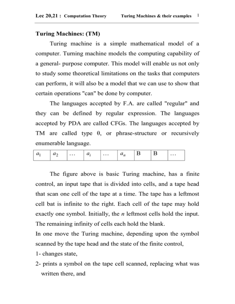
The figure above is basic Turing machine, has a finite
control, an input tape that is divided into cells, and a tape head
that scan one cell of the tape at a time. The tape has a leftmost
cell bat is infinite to the right. Each cell of the tape may hold
exactly one symbol. Initially, the n leftmost cells hold the input.
The remaining infinity of cells each hold the blank.
In one move the Turing machine, depending upon the symbol
scanned by the tape head and the state of the finite control,
1- changes state,
2- prints a symbol on the tape cell scanned, replacing what was
written there, and
Lec 20,21 : Computation Theory
Turing Machines & their examples
2
3- moves its head left or right one cell
Note that the difference between a Turing machine and a twoway finite automation lies in the ability to change symbols on its
tape.
Formally, a Turing machine (TM) is denoted:
M  (Q, , , t , q , B, F )
Where
Q is the finite set of "states",
 is the finite set of a allowable "tape symbols",
B, a symbol of  , is the "blank",
 , a subset of  not including B, is the set of "input symbols"
T, is the next move function, a mapping from Q   to
Q    {L, R},
q , in Q is the "start state ",
F  Q is the set of "final states", or called "HALT states" that
cause execution to terminate when we enter them.
The "language accepted" by M, denoted L(M), is the set of those
word in * that cause M to enter a final state.
Lec 20,21 : Computation Theory
Turing Machines & their examples
3
First Example TM
y\y,R
n n
L={0 1 }
B\B,R
q5
q4
0\0,R
y\y,R
0\x,R
q0
q1
1\y,L
x\x,R
q2
q0
y\y,L
x\x,R
0\0,L
q3
0\0,L

Q

F
M  ({q , q1 , q2 , q3 , q4 },{0,1, B},{x, y},{q4 }) and Transition functions are:
t (q ,0)  (q1 , X , R)
t (q2 ,0)  (q3 ,0, L)
t (q1 ,Y )  (q1 ,Y , R)
t ( q 2 , X )  ( q 4 , X , R)
t (q1 ,0)  (q1 ,0, R)
t (q2 , Y )  (q2 , Y , L)
t (q1 ,1)  (q2 , Y , L)
t (q3 ,0)  (q3 ,0, L)
t (q3 , x)  (q0 , x, R)
t ( q 4 , Y )  ( q 4 , Y , R)
t (q4 , B)  (q5 , B, R)
A computation of M on input 0011 is:
q 0011  Xq1 011  X 0q111  Xq2 0Y1 
q3 X 0Y1  Xq  0Y1  XXq1Y1  XXXq 11 
Lec 20,21 : Computation Theory
4
Turing Machines & their examples
XXq2YY  Xq2 XYY  XXq4 XY  XXYq4Y 
XXYYq4  XXYYBq5
Second Example TM
L= {WWr W={a,b}+}
a\a,L
b\b,L
a\a,R
b\b,R
q1
B\B,L
a\B,R
q0
a\B,L
q2
B\B,R
B\B,R
q7
q0
a\a,L
b\b,L
b\B,R
q4
a\a,R
b\b,R
q3
B\B,R
B\B,L
q5
b\B,L
q6