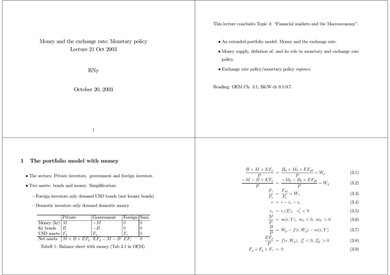
This lecture concludes Topic 4: “Financial markets and the Macroeconomy”.
Money and the exchange rate; Monetary policy
Lecture 21 Oct 2003
• An extended portfolio model: Money and the exchange rate.
• Money supply, defintion of, and its role in monetary and exchange rate
policy.
• Exchange rate policy/monetary policy regimes.
RNy
Reading: OEM Ch. 3.1, B&W ch 9.1-9.7.
October 20, 2003
1
1
The portfolio model with money
• The sectors: Private investors, government and foreign investors
• Two assets: bonds and money. Simplification:
— Foreign investors only demand USD bonds (not kroner bonds)
— Domestic investors only demand domestic money
Money (kr)
Kr bonds
USD assets
Net assets
Private
M
B
Fp
M + B + EFp
Government
−M
−B
Fg
EFg − M − B
Foreign
0
0
F∗
EF∗
Sum
0
0
0
0
Tabell 1: Balance sheet with money (Tab 3.1 in OEM)
B + M + EFp
P
−M − B + EFg
P
F∗
P∗
r
ee
M
P
B
P
EFp
P
Fg + Fp + F∗
B0 + M0 + EFp0
= Wp
P
−M0 − B0 + EFg0
=
= Wg
P
F∗0
=
= W∗
P∗
= i − i∗ − ee
=
= ee(E),
e0e
<0
(3.1)
(3.2)
(3.3)
(3.4)
(3.5)
= m(i, Y ), mi < 0, mY > 0
(3.6)
= Wp − f (r, Wp) − m(i, Y )
(3.7)
0
>0
= f (r, Wp), fr0 < 0, fW
(3.8)
= 0
(3.9)
Endogenous: Wg , Wp, W∗, F∗,Fp, r, ee + 3 depending on regime.
(note: 10 endogenous variables, not 12, since only 10 independent equation).
Exogenous: i∗, Y, P, P∗, M0, B0, Fp0, Fgo,F∗
Regime
Fixed exchange rate
I Fixed interest rate
II No sterilization
III Full sterilization
Floating exchange rate
IV Fixed interest rate
V No sterilization
VI Full sterilization
Exogenous Endogenous
E, i
E, B,
E, M
Fg , M, B
Fg , i, M
Fg , i, B
Fg , i
Fg , B
Fg , M
E, M, B
E, i, M
E, i, B
Tabell 2: Policy regimes (Tab 3.2)
We interpret the exogenous variables (in the table) as either targets of economic policy, or instruments which are “set aside” to attain other target
variables, which are not specified in the portfolio model.
We will not analyse in detail all 6 regimes, leave that to ECON 4330.
Will instead spend some time on regime III, and then concentrate on the float
Money supply and sterilization
Money demand is represented in the model by a separate equation.
regimes.
But first, need to clarify money supply and sterilization
What about the supply of money?
Being a stock variable, total money supply is unaffected by e.g., the government surplus/deficit (flow) in the short run.
The portfolio model is a short run model, still some of the regimes in table
2 has M as endogenous? Is this an inconsistency? The answer is no, since
money supply is linked to other stock variables.
Definition: Sterilization
Consider (3.2):
−M − B + EFg −M0 − B0 + EFg0
=
= Wg
P
P
Assuming a fixed exchange rate regime, and noting that P and Wg are constants within the short period of the model, we derive form (3.2):
(3.10)
dM = E dFg − dB
where dM = M − M0, dFg = Fg − Fg0 and dB = B − Bg0.
The degree of sterilization in monetary policy denotes how much B is changed
(by market operations) when there is a change in Fg . Formally,
dB
EdF g
s = 1: Full sterilization. s = 0: No sterilization.
s=
Regime II (fixed): The link dFg → dM is not sterilized by increased bonds
sales, i.e.,
(3.10) is the fundamental money-supply function of an open economy: It
links money supply to changes in other stocks. In particular: if the supply
dB
=0
EdFg
of domestic bonds is fixed (dB = 0), there is a direct link to from foreign
Regime III (fixed): The link is broken (dFg 9 dM), i.e., domestic money
currency reserves to the money supply.
supply is “insulated” from the market for exchange rate.
dB
=1
EdFg
Regime V and VI, (float) are equivalent as long the there is a “clean float”.
What kind of money?
As long as dFg = 0, constant M is only possible with B constant (and vice
versa).
Economists use several definitions of money. M in the portfolio model can be
interpreted in two ways:
However, for a managed float, with interventions
i) As the stock of base money, M0, notes and coins issued by the central bank,
or
• Regime V: dM = EdFg
• Regime VII: dM = 0 and dB = EdFg (s = 1).
ii) since one function of private bank is to create money, we can also reason
as if M corresponds to a broader definition of money, M 1, M2 or M3.
The second, and more interesting, interpretation builds on the money (and
credit) multiplier: The basic intuition is that each time a bank issues a loan,
reserve requirements also creates a deposit (which goes into the wider money
measures).
B&W’s chapter 9, makes for interesting, but cursory reading on this subject.
Solving the model: A two step procedure
Step 1: Determining the interest rate
1. Find out how the interest rate is determined.
Regime I and IV: i is exogenous. Either it is a target variable on its own,
2. Given the solution for the interest rate, find the solu-
or it is determined outside the model, for example it is used as an instrument
tion for E or Fg from the equilibrium condition in the
to attain some other target variable, not specified in the portfolio model.
market for foreign exchange.
Regime III, V and VI (clean float): i is determined in the money market
M = P m(i, Y )
(3.12)
with M exogenous. Cf Figure 3.2. (See appendix for Regime II, fixed without
sterilization)
Step 2: The market for foreign exchange (and overall
equilibrium).
For a given equilibrium level (or exogenous as in R I and IV), Fg , or E,is
determined by the equilibrium condition
(3.14)
Fg = −F∗0 −
P
B0 + M0 + EFp0
f (i − i∗ − ee(E),
)
E
P
(we have used F∗ = F∗0). Note that
∂Fg
>0
∂E
under the same set of condition as in the simplest model (OEM Ch. 1).
Note also that
P
∂Fg
= − fr > 0, relevant for fix-regimes
∂i
E
P fr
∂E
=
< 0, relevant for float
∂i
(1 − fW )Fp0 + P e0efr
∂E/∂i is achieved by implicit derivation of (3.14), and is the slope of the
Ei-curve introduced in the previous lecture (see appendix B) .
2
Examples of monetary policy analysis
Regime III
Hence, in order to increase M by 1bill, the CB needs to buy bonds for more
than 1bill, since reserves are worn down (dFg < 0) when the S-curve of foreign
currency is shifted leftwards:
Assume that the government wants monetary expansion (e.g., to stimulate
the real economy).
In this regime: Uses market operations to achieve an increase in the targeted
(3.21)
dFg
dFp dF∗
P di
1 fr
<0
= −[
+
] = − fr
=−
dM
dM dM
E dM
E mi
Role of capital mobility: From (3.21)
dFg
1 fr
=−
dM
E mi
money supply (consistent with this, M is exogenous in the model, B, the
instrument is endogenous).
→
−fr0 →∞
−∞
implying that full sterilization is a logical impossibility when capital mobility
Effect on i from money market equilibrium (3.12)
is perfect: The central bank cannot control the money supply.
di
1
(3.19)
=
< 0.
dM P mi
Effect on B (use equation (3.13)):
If there is full capital mobility: monetary policy becomes ineffective.
(3.20)
fr + mi
di
di
dB
< −1
= P [−fr
− mi
]=−
dM
dM
dM
mi
Regime V/VII, clean float
An important “left out” regime
dM > 0 is achieved by market operations dB = −dM .
The book does not cover one of the regimes that characterized both Sweden
Effect: i & (money market) and E % (market for foreign exchange).
of both Fg and E exogenous with i endogenous and M endogenous.
Effect on E depend on degree of capital mobility (how?)
and Norway in the 1990s (as well as many other countries): namely the case
This allows maintaining fixed E as target, while freezing Fg at a certain level.
In the model, i is determined by the equilibrium condition for the market for
An appendix provides a cursory analysis of “dirty float” regimes.
foreign exchange.
Graphically, the regime can be analysed using the Ei-curve along with a the
money-market graph.
(Short-run) interest rates can become high during periods of speculative attack
(cf graphs of Swedish and Norwegian interest rates in 1992).
Model formulation with perfect capital mobility
A
No rationale for separate asset demand functions. The models reduces to
i is determined in the domestic bonds market: The equilibrium condition
M
= m(i, Y ), mi < 0, mY > 0
P
r = i − i∗ − ee(E) = 0
Interest rate determination in Regime II
(3.22)
follows from (3.1), (3.4) and (3.5) and (3.7)
(3.23)
(3.13)
with i and M endogenous in a fixed exch rate regimes, and i and E endogenous
B M0 + B0 + EFp0
M0 + B0 + EFp0
=
−f (i−i∗ −ee(E),
)−m(i, Y ).
P
P
P
The right hand side of (3.12) defines the demand function
in a float regime.
B d = B(i, E, Y, P, i∗, B0, M0, Fp0), Bi > 0,
Which regimes can be operational in this case?
which is increasing in i: The higher i, the less demand for foreign exchange,
1. Using the interest rate to target E (requires e0e 6= 0)
2. Clean float, with M−targeting
3. Dirty float with interventions (see an appendix).
4. Clean float with targeting of some variable outside this model (e.g., in-
and the less demand for money. Formally
∂B d
= −P (fr + mi) > 0
∂i
flation). i as instrument.
B
The slope of the Ei-curve
Solving for ∂E/∂i, and noting that Fp = P f (r, WP )/E and setting Fp = Fp0
(since both Fg and F∗ are constant), we obtain
P fr
∂E
< 0.
=
∂i
(1 − fW )Fp0 + P e0efr
In the basic portfolio model (previous lecture) we derived the partial derivative ∂E/∂i from the derivatives for Si and SE of the supply function of
In terms of the model in Chapter 1 of OEM:
foreign currency. Here we calculate ∂E/∂i from (3.14). Of course, the two
approaches amount to the same thing, as the underlying relationship is the
γ = (1 − fW )
market equilibrium condition. Some details: Implicit derivation of (3.14)
κ = −fr ,
gives:
0=−
"
P f (r, Wp) ∂E
∂i
E2
½
¾#
P
Fp0 ∂E
0 ∂E
+
fr (1 − ee ) + fW
E
∂i
P ∂i
EFp0
,
P
thus
−P κ
∂E
=
∂i
(1 − fW )Fp0 EP EP − P e0eκ
−κ
= 1
γ E − e0eκ
−1
= γ
0
κE − ee
• “minus”, since dM = −dB, from the money demand function (3.10),
the same expression as in (1.24).
dM > 0 =⇒ dB < 0.
C
• The market equilibrium glides down along the B d-curve in Figure 3.2 in
Monetary policy: Fixed exchange rate without
sterilization
The money supply is not controlled (M is endogenous). Monetary expansion
means that the government succeed in reducing private net stocks of bonds:
The central banks buys bonds from the public (“open market operation”).
−
Assume that the initial increase in M was 1billion (if dB = −1bill). In the
new equilibrium:
dM
mi
1
= P mi
=
<1
dB
P (fr + mi) (f r + mi)
since Fg is reduced to restore equilibrium in the market for foreign exchange.
(3.17)
−
dFg
dM
fr
= −[
+ 1] = −[
] < 0.
dB
dB
(fr + mi)
(Supply of foreign currency is reduced by i &. In order to keep E constant,
The effect on i is found from (3.13)
(3.16)
OEM.
(3.18)
di
1
=
<0
dB P (fr + mi)
−
Fg must fall by the same amount).
In the analysis of Regime III, full sterilization, we saw that monetary policy
D
Dirty float regimes
had no effect on the interest rate if capital mobility is perfect.
How is the regime with no attempt to sterilise affected? From (3.17)
−
dM
mi
=
dB
(fr + mi)
→
−fr →∞
0.
since −fr → ∞ means that Fg falls by the same amount as Bs. From (3.18):
−E
This supplements the discussion of the case of a clean float above:
dFg
fr
1
= −[
] = −[
] → −1.
dB
(fr + mi)
(1 + mi/fr ) −fr0 →∞
Intervention without sterilization
dM = EdFg > 0 and dB = 0. Leads to i & and E %. Foreign exchange
Hence, again as a result of the link between foreign currency reserves and the
market: Negative horizontal shift in the S-curve, and demand increases. Both
money supply, perfect capital mobility makes monetary policy ineffective also
imply higher E (depreciation). The policy work also with high capital mobil-
in Regime II. Formally:
ity, since i is affected.
−
di
1
=
dB P (fr + mi)
→
−fr0 →∞
0
Sterilized intervention
dB = EdFg > 0, dM = 0. No change in i. But E % since Fg increases
(demand for foreign exchange).
Perfect capital mobility takes away the effects of sterilized interventions, the
S-curve becomes horizontal..