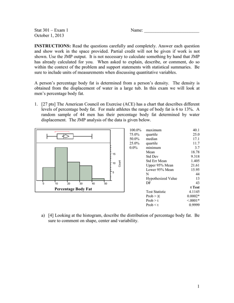
Stat 301 – Exam 1
October 1, 2013
Name: ________________________
INSTRUCTIONS: Read the questions carefully and completely. Answer each question
and show work in the space provided. Partial credit will not be given if work is not
shown. Use the JMP output. It is not necessary to calculate something by hand that JMP
has already calculated for you. When asked to explain, describe, or comment, do so
within the context of the problem and support statements with statistical summaries. Be
sure to include units of measurements when discussing quantitative variables.
A person’s percentage body fat is determined from a person’s density. The density is
obtained from the displacement of water in a large tub. In this exam we will look at
men’s percentage body fat.
1. [27 pts] The American Council on Exercise (ACE) has a chart that describes different
levels of percentage body fat. For male athletes the range of body fat is 6 to 13%. A
random sample of 44 men has their percentage body fat determined by water
displacement. The JMP analysis of the data is given below.
100.0%
75.0%
50.0%
25.0%
0.0%
10
5
0
10
20
30
40
Percentage Body Fat
50
Count
15
maximum
quartile
median
quartile
minimum
Mean
Std Dev
Std Err Mean
Upper 95% Mean
Lower 95% Mean
N
Hypothesized Value
DF
Test Statistic
Prob > |t|
Prob > t
Prob < t
40.1
25.0
17.1
11.7
3.7
18.78
9.318
1.405
21.61
15.95
44
13
43
t Test
4.1145
0.0002*
<.0001*
0.9999
a) [4] Looking at the histogram, describe the distribution of percentage body fat. Be
sure to comment on shape, center and variability.
1
b) [3] Looking at the box plot, are their any potential outliers? How do you know
this? If so, what is (are) the associated percentage body fat(s)?
c) [8] Could this sample be from a population of athletes? Test the hypothesis that
the population mean percentage body fat is 13% versus an alternative that the
population mean percentage fat is greater than 13%. Be sure to give the null and
alternative hypothesis using appropriate statistical notation, value of the test
statistic, P-value, decision and reason for reaching that decision and a conclusion
in the context of the problem. For this problem use the usual significance level of
0.05.
d) [4] Give the values for the 95% confidence interval for the population mean
percentage body fat. Explain briefly why this confidence interval is consistent
with the test of hypothesis you did in c).
2
e) [4] Construct a 95% prediction interval for the percentage body fat of a randomly
selected man. Note: the appropriate value of t* is 2.0167.
f) [4] What is the difference in interpretation between the confidence interval in d)
and the prediction interval in e)?
2. [33 pts] The random sample of 44 men includes 24 men who are under 40 years of
age and 20 men who are 40 to 55 years of age. The JMP analysis appears below.
50
Rsquare
Adj Rsquare
Root Mean Square Error
Mean of Response
Observations (or Sum Wgts)
BodyFat
40
30
20
t Test
Difference
Std Err Dif
Upper CL Dif
Lower CL Dif
Confidence
10
0 40 to 55
under 40
Age Group
Level
40 to 55
under 40
Number
20
24
Mean
23.9650
14.4583
Std Dev
10.2158
5.7648
Std Err Mean
2.2843
1.1767
0.264098
0.246576
8.087709
18.77955
44
Assuming equal variances
9.507 t Ratio
3.88237
2.449 DF
42
14.448 Prob > |t|
0.0004*
4.565 Prob > t
0.0002*
0.95 Prob < t
0.9898
Lower 95%
19.184
12.024
Upper 95%
28.746
16.893
a) [5] Compare the percentage body fat of 40 to 55 year old men to that of the men
under 40. Be sure to compare centers, variability and mention if there are any
potential outliers in either group.
3
b) [3] What is the value of sp, the pooled estimate of the common standard deviation,
σ?
c) [8] Test the hypothesis that there is no difference between the population mean
percentage body fat of 40 to 55 year old men and the population mean percentage
body fat of men under 40 years old. Be sure to give the null and alternative
hypothesis using clearly understood statistical symbols, value of the test statistic,
P-value, decision and reason for reaching that decision and a conclusion in the
context of the problem.
d) [5] Give the 95% confidence interval for the difference in population mean
percentage body fat. What does this say about how much the population mean
percentage body fat of men 40 to 55 years old differs from that of men under 40
years old?
e) [4] Is the condition of equal population standard deviations, σ, satisfied for these
data? Support your answer.
4
Below is the JMP output for the distribution of the two-sample residuals.
0.95
Normal Quantile Plot
1.64
1.28
0.85
0.67
0.0
0.75
0.60
0.45
0.30
-0.67
0.20
-1.28
0.10
-1.64
0.05
5
-20
-15
-10
-5
0
5
10
15
Count
10
20
Residual
f) [3] Looking at the normal quantile plot describe what you see and what this tells
you about the condition that random errors are normally distributed.
g) [3] Looking at the box plot compare the median to the mean? What does this
comparison indicate about the shape of the distribution of residuals?
h) [2] Looking at the histogram, where is the mound? How would you describe the
shape of the distribution of residuals?
5
3. [40] Measuring percentage body fat by displacement of water is a time consuming
process that requires the individual to be naked. Could a less time consuming and
invasive measurement, like the circumference of a man’s abdomen (cm), be used to
predict the percentage body fat? Below is JMP output looking at the relationship
between abdomen circumference and percentage body fat.
50
Summary of Fit
RSquare
RSquare Adj
Root Mean Square Error
Mean of Response
Observations (or Sum Wgts)
BodyFat
40
30
20
0.706645
0.699660
5.10637
18.77955
44
10
0
50
100
1
Abdomen
Parameter Estimates
Term
Estimate Std Error
Intercept
–41.19
6.012
Abdomen (cm)
0.648
0.0644
t Ratio Prob>|t| Lower 95%
–6.85 <.0001*
–53.32
10.06 <.0001*
0.518
Upper 95%
–29.06
0.778
a) [3] Describe the general relationship between abdomen circumference and
percentage body fat. Use complete sentences and say something about direction,
form, strength and unusual values.
b) [3] Give the equation of the least squares regression line relating percentage body
fat to the abdomen circumference.
c) [2] Use the equation in b) to predict the percentage body fat for a man with
abdomen circumference of 110 cm.
6
d) [5] Calculate a 95% prediction interval for a man with abdomen circumference of
110 cm. Note t* = 2.01081. Note: the sample mean abdomen circumference is
92.6 cm and the sample variance of abdomen circumference is 146.21 cm2.
e) [5] Give an interpretation of the estimated slope coefficient within the context of
the problem.
f) [3] Why doesn’t the intercept have an interpretation within the context of the
problem?
g) [3] Give the value of R2 and an interpretation of that value within the context of
the problem.
h) [2] Give the value of the estimate of the random error standard deviation, σ.
7
i) [6] Report the 95% confidence interval for the slope. Use this interval to test for a
statistically significant relationship between percentage body fat and abdomen
circumference.
j)
[4] Describe what you see in the plot of residuals versus predicted body fat.
What does this plot tell you about the adequacy of the linear model?
10
BodyFat Residual
5
0
-5
-10
0
10
20
30
40
50
BodyFat Predicted
k) [4] Comment on the condition of normally distributed random errors. Be sure to
support your comments by referring to the normal quantile plot of residual.
5
0
0.9
0.9
0.8
0.7
0.6
0.5
0.4
0.3
0.2
0.1
-10
0.1
-5
0.0
BodyFat Residual
10
Normal Quantile
8