1.1 Latent Variable Models - Introduction
1.1
2
Latent Variable Models - Introduction
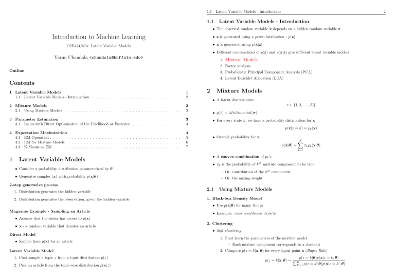
• The observed random variable x depends on a hidden random variable z
Introduction to Machine Learning
• z is generated using a prior distribution - p(z)
• x is generated using p(x|z)
CSE474/574: Latent Variable Models
• Different combinations of p(z) and p(x|z) give different latent variable models
Varun Chandola <chandola@buffalo.edu>
1. Mixture Models
2. Factor analysis
Outline
3. Probabilistic Principal Component Analysis (PCA)
4. Latent Dirichlet Allocation (LDA)
Contents
1 Latent Variable Models
1.1 Latent Variable Models - Introduction . . . . . . . . . . . . . . . . . . . . . . . . . . . . .
1
2
2 Mixture Models
2.1 Using Mixture Models . . . . . . . . . . . . . . . . . . . . . . . . . . . . . . . . . . . . . .
2
2
3 Parameter Estimation
3.1 Issues with Direct Optimization of the Likelihood or Posterior . . . . . . . . . . . . . . . .
3
4
4 Expectation Maximization
4.1 EM Operation . . . . . . . . . . . . . . . . . . . . . . . . . . . . . . . . . . . . . . . . . . .
4.2 EM for Mixture Models . . . . . . . . . . . . . . . . . . . . . . . . . . . . . . . . . . . . .
4.3 K-Means as EM . . . . . . . . . . . . . . . . . . . . . . . . . . . . . . . . . . . . . . . . . .
4
5
6
7
2
Mixture Models
• A latent discrete state
z ∈ {1, 2, . . . , K}
• p(z) ∼ M ultinomial(π)
• For every state k, we have a probability distribution for x
p(x|z = k) = pk (x)
1
Latent Variable Models
• Consider a probability distribution parameterized by θ
• Overall, probability for x
p(x|θ) =
1. Distribution generates the hidden variable
2. Distribution generates the observation, given the hidden variable
πk pk (x|θ)
k=1
• A convex combination of pk ’s
• πk is the probability of k th mixture component to be true
– Or, contribution of the k th component
• Generates samples (x) with probability p(x|θ)
2-step generative process
K
X
– Or, the mixing weight
2.1
Using Mixture Models
1. Black-box Density Model
• Use p(x|θ) for many things
Magazine Example - Sampling an Article
• Example: class conditional density
• Assume that the editor has access to p(x)
• x - a random variable that denotes an article
Direct Model
• Sample from p(x) for an article
Latent Variable Model
1. First sample a topic z from a topic distribution p(z)
2. Pick an article from the topic-wise distribution p(x|z)
2. Clustering
• Soft clustering
1. First learn the parameters of the mixture model
– Each mixture component corresponds to a cluster k
2. Compute p(z = k|x, θ) for every input point x (Bayes Rule)
p(z = k|θ)p(x|z = k, θ)
p(z = k|x, θ) = PK
0
0
k0 =1 p(z = k |θ)p(x|z = k , θ)
3. Parameter Estimation
3
3.1 Issues with Direct Optimization of the
Likelihood or Posterior
3.1
200
4
Issues with Direct Optimization of the Likelihood or Posterior
• For direct optimization, we find parameters that maximize (log-)likelihood (or (log-)posterior)
150
100
• Easy to optimize if zi were all known
50
• What happens when zi ’s are not known
0
[2, 4) [4, 6) [6, 8)[8, 10)[10, 12)
[12, 14)
– Likelihood and posterior will have multiple modes
– Non-convex function - harder to optimize
250
200
150
4
100
Expectation Maximization
• Recall the we want to maximize the log-likelihood of a data set with respect to θ:
50
0
[0, 5)
[5, 10)
[10, 15)
θ̂ = maximize `(θ)
θ
3
• Log-likelihood for a mixture model can be written as:
Parameter Estimation
Simple Parameter Estimation
`(θ) =
• Given: A set of scalar observations
x1 , x2 , . . . , xn
=
2. Make choice of the form of the probability distribution (Gaussian)
3. Estimate parameters from the data using MLE or MAP (µ and σ)
`(θ) =
=
• Single mode is not sufficient
– zi = 2 means that xi comes from second mixture component
• Issue: zi ’s are not known beforehand
• Need to explore 2N possibilities
N
X
i=1
N
X
K
X
k=1
log p(xi |θ)
log
i=1
• In reality data is generated from two Gaussians
– zi = 1 means that xi comes from first mixture component
log
"
#
p(zk )pk (xi |θ)
Note that the above equation for log-likelihood is for mixture models only. In general, it maybe written
as:
When Data has Multiple Modes
• What if we knew zi ∈ {1, 2}?
log p(xi |θ)
• Hard to optimize (a summation inside the log term)
In the above example we choose the random variable x to be distributed as a Gaussian random variable.
• How to estimate µ1 , σ1 , µ2 , σ2 ?
i=1
N
X
i=1
• Task: Find the generative model (form and parameters)
1. Observe empirical distribution of x
N
X
=
N
X
log
i=1
"
"
X
∀zk
X
∀zk
#
p(xi , zk |θ)
#
p(zk )p(xi |zk , θ)
• Repeat until converged:
1. Start with some guess for θ and compute the most likely value for zi , ∀i
2. Given zi , ∀i, update θ
• Does not explicitly maximize the log-likelihood of mixture model
• Can we come up with a better algorithm?
– Repeat until converged:
Obviously, if zi ’s were known, you can create two data sets corresponding to the two values that zi can
take, and then estimate parameters for each set.
1. Start with some guess for θ and compute the probability of zi = k, ∀i, k
2. Combine probabilities to update θ
4.1 EM Operation
5
4.2 EM for Mixture Models
6
Steps in EM
• EM is an iterative procedure
• Start with some value for θ
• At every iteration t, update θ such that the log-likelihood of the data goes up
– Move from θ t−1 to θ such that:
`(θ) − `(θ t−1 )
is maximized
• Complete log-likelihood for any LVM
`(θ) =
N
X
i=1
log p(xi , zi |θ)
• Cannot be computed as we do not know zi
4.2
Expected complete log-likelihood
Q(θ, θ t−1 ) = E[`(θ|D, θ t−1 )]
• Expected value of `(θ|D, θ t−1 ) for all possibilities of zi
EM for Mixture Models
• EM formulation is generic
• Calculating (E) and maximizing (M) Q() needs to be done for specific instances
Q for MM
Recall that expected value of a function f (x) for a random variable x is given by:
X
E[f (x)] =
f (x0 )p(x0 )
Q(θ, θ
t−1
) = E
x0
=
If x is continuous, the sum is replaced by an integral
Z
E[f (x)] = f (x)p(x)dx
rik , p(zi =
"
N
X
#
log p(xi , zi |θ)
i=1
N X
K
X
rik log πk +
i=1 k=1
k|xi , θ t−1 )
N X
K
X
i=1 k=1
rik log p(xi |θk )
In the case of EM, we are interested in computing the expected value over all possibilities of z. The
probability of each possibility is computed using the current estimate θ t−1 .
The quantity rik can be thoughts of as the responsibility that cluster k takes for data point xi in iteration
t.
4.1
E-Step
EM Operation
• Compute rik , ∀i, k
1. Initialize θ
2. At iteration t, compute Q(θ, θ
t−1
)
3. Maximize Q() with respect to θ to get θ t
4. Goto step 2
• Compute Q()
rik = p(zi = k|xi , θ t−1 )
πk p(xi |θkt−1 )
= P 0
0t−1
)
k0 πk p(xi |θk
M-Step
• Maximize Q() w.r.t. θ
• θ consists of π = {π1 , π2 , . . . , πK } and θ = {θ1 , θ2 , . . . , θK }
4.3 K-Means as EM
7
• For Gaussian Mixture Model (GMM) (θk ≡ (µk , Σk )):
(1)
µk
(2)
Σk
4.3
K-Means as EM
1 X
rik
N i
P
rik xi
= Pi
rik
P i
>
r
i ik xi xi
P
− µk µ>
=
k
r
ik
i
πk =
(3)
• Similar to GMM
1. Σ = σ 2 ID
2. πk =
1
K
3. The most probable cluster for xi is computed as the prototype closest to it (hard clustering)
References