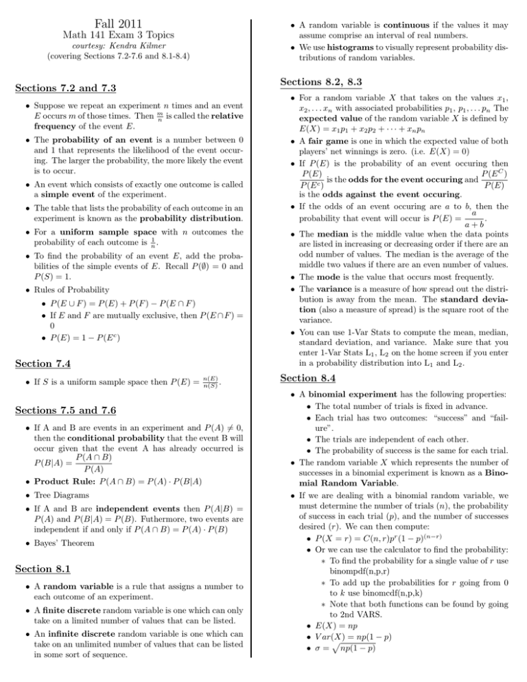
Fall 2011
• A random variable is continuous if the values it may
assume comprise an interval of real numbers.
• We use histograms to visually represent probability distributions of random variables.
Math 141 Exam 3 Topics
courtesy: Kendra Kilmer
(covering Sections 7.2-7.6 and 8.1-8.4)
Sections 8.2, 8.3
Sections 7.2 and 7.3
• Suppose we repeat an experiment n times and an event
E occurs m of those times. Then m
n is called the relative
frequency of the event E.
• The probability of an event is a number between 0
and 1 that represents the likelihood of the event occuring. The larger the probability, the more likely the event
is to occur.
• An event which consists of exactly one outcome is called
a simple event of the experiment.
• The table that lists the probability of each outcome in an
experiment is known as the probability distribution.
• For a uniform sample space with n outcomes the
probability of each outcome is n1 .
• To find the probability of an event E, add the probabilities of the simple events of E. Recall P (∅) = 0 and
P (S) = 1.
• Rules of Probability
• P (E ∪ F ) = P (E) + P (F ) − P (E ∩ F )
• If E and F are mutually exclusive, then P (E ∩ F ) =
0
• P (E) = 1 − P (E c )
Section 7.4
• If S is a uniform sample space then P (E) =
n(E)
n(S) .
Sections 7.5 and 7.6
• If A and B are events in an experiment and P (A) 6= 0,
then the conditional probability that the event B will
occur given that the event A has already occurred is
P (A ∩ B)
P (B|A) =
P (A)
• Product Rule: P (A ∩ B) = P (A) · P (B|A)
• Tree Diagrams
• If A and B are independent events then P (A|B) =
P (A) and P (B|A) = P (B). Futhermore, two events are
independent if and only if P (A ∩ B) = P (A) · P (B)
• Bayes’ Theorem
Section 8.1
• A random variable is a rule that assigns a number to
each outcome of an experiment.
• A finite discrete random variable is one which can only
take on a limited number of values that can be listed.
• An infinite discrete random variable is one which can
take on an unlimited number of values that can be listed
in some sort of sequence.
• For a random variable X that takes on the values x1 ,
x2 , . . . xn with associated probabilities p1 , p1 , . . . pn The
expected value of the random variable X is defined by
E(X) = x1 p1 + x2 p2 + · · · + xn pn
• A fair game is one in which the expected value of both
players’ net winnings is zero. (i.e. E(X) = 0)
• If P (E) is the probability of an event occuring then
P (E C )
P (E)
is the odds for the event occuring and
c
P (E )
P (E)
is the odds against the event occuring.
• If the odds of an event occuring are a to b, then the
a
probability that event will occur is P (E) =
.
a+b
• The median is the middle value when the data points
are listed in increasing or decreasing order if there are an
odd number of values. The median is the average of the
middle two values if there are an even number of values.
• The mode is the value that occurs most frequently.
• The variance is a measure of how spread out the distribution is away from the mean. The standard deviation (also a measure of spread) is the square root of the
variance.
• You can use 1-Var Stats to compute the mean, median,
standard deviation, and variance. Make sure that you
enter 1-Var Stats L1 , L2 on the home screen if you enter
in a probability distribution into L1 and L2 .
Section 8.4
• A binomial experiment has the following properties:
• The total number of trials is fixed in advance.
• Each trial has two outcomes: “success” and “failure”.
• The trials are independent of each other.
• The probability of success is the same for each trial.
• The random variable X which represents the number of
successes in a binomial experiment is known as a Binomial Random Variable.
• If we are dealing with a binomial random variable, we
must determine the number of trials (n), the probability
of success in each trial (p), and the number of successes
desired (r). We can then compute:
• P (X = r) = C(n, r)pr (1 − p)(n−r)
• Or we can use the calculator to find the probability:
∗ To find the probability for a single value of r use
binompdf(n,p,r)
∗ To add up the probabilities for r going from 0
to k use binomcdf(n,p,k)
∗ Note that both functions can be found by going
to 2nd VARS.
• E(X) = np
• V ar(X)
p = np(1 − p)
• σ = np(1 − p)