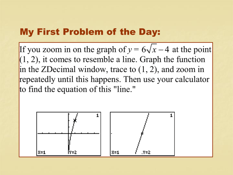
My First Problem of the Day:
If you zoom in on the graph of y = 6 x  4 at the point
(1, 2), it comes to resemble a line. Graph the function
in the ZDecimal window, trace to (1, 2), and zoom in
repeatedly until this happens. Then use your calculator
to find the equation of this "line."
Point-Slope Equation of a Line:
y  y1  m( x  x1 )
Linearization of f at x = a:
y  f (a)  f (a)( x  a)
or
y  f (a)  f (a)( x  a)
This simple equation is the basis for:
Instantaneous rate of change
Differentials
Linear approximations
Newton’s Method for Finding Roots
Rules for Differentiation
Slope Fields
Euler’s Method
L’Hopital’s Rule
What is Instantaneous Rate of Change?
If a rock falls 20 feet in 2 seconds, its
average velocity during that time period
is easily measured:
20 feet
 10 ft/sec
2 sec
But what if we capture that rock at a
moment in time and ask for its
instantaneous velocity at that single
moment? What is the logical reply?
0 feet 0
 ft/sec
0 sec 0
Obviously, traditional algebra fails us
when it comes to instantaneous rate
of change.
feet
seconds
But if we graph the rock’s position as a
function of time, we see that velocity is
the same as slope. Instantaneous
velocity is just the slope of the
zoomed-in picture – which is linear!
That’s what differentials are all about.
Since the derivative is the slope of the
curve at a point, there is no true Δy or
Δx…but there is a slope. So we write:
y dy
lim

x 0 x
dx
If we zoom in on a differentiable
curve, because it is locally linear,
Δy/ Δx is essentially constant. That
makes dy/dx defensible as something
other than 0/0.
If we zoom in at a point (a, f(a)):
y
lim
 f (a)
x 0 x
So… if (x, y) is close to (a, f(a)),
y  f (a)
 f (a)  y  f (a)  f (a)( x  a)
xa
There’s that equation again!
This is the basis for linear
approximations. For example, here is
Problem of the Day #23:
Find the linearization of f ( x )  x at x = 100 and use
it to approximate 101 . Use f  to predict whether the
approximation will be slightly smaller or slightly
larger than the actual value.
1
y  100 
 x  100 
2 100
1
 y  10  101  100   y  10.05
20
The Good News: Modern students can
check how close this approximation
is by using a calculator.
The Bad News: Modern students do
not appreciate how much these
approximation tricks meant to their
ancestors.
Another such method is Newton’s
Method for approximating roots. Here is
Problem of the Day #22:
The line shown is tangent to the graph of y = f(x) at the
point (a, f(a)).
(a, f(a))
(a) Find an equation of the line.
(b) Find the x-intercept of this line in terms of a.
y  f (a )  f (a )( x  a )
0  f (a )  f (a )( x  a )
f (a)
xa
f (a )
Then we name this x-intercept b.
Using (b, f(b)) as the new point, I
have them repeat the process. Clever
students quickly write:
f (b)
xb
f (b)
(a, f(a))
Eventually this process will zoom in
on an x-intercept of the curve. This
is Newton’s Method for
approximating roots of equations.
For example, let us find a root of the
equation sin x = 0. Start with a guess
of a = 2.
sin a
xa
 a  tan a
cos a
2
Local linearity even led to the discovery
of the differentiation rules. For
example, here’s the product rule.
Zoom in on a product function uv until it
looks linear. The slope will be the
derivative of uv.
(x + dx, (u + du)(v + dv))
d(uv)
(x, uv)
dx
d (uv) (u  du )(v  dv )  uv

dx
dx
uv  udv  vdu  dudv  uv

dx
udv  vdu  dudv

dx
dv
du
dv
u v
 du
dx
dx
dx
A slope field is all about local linearity.
dy
 x y
dx
At each point (x, y) the differential
equation determines a slope. This is
the very essence of point-slope!
Here is Problem of the Day #37:
Suppose y = f(x) satisfies the differential equation
dy
 x  y . Find the linearization of f at the point (1, 1)
dx
and use it to approximate f(1.1). Then use the
linearization at the new point to approximate f(1.2).
This is Euler’s
Method. The
picture at the
right shows how
it works.
dy
dx
( x  x , y  y )
(x, y)
 dy 
y    x
 dx 
Slope
x
You start with a point on the curve.
Find the slope, dy/dx.
Now move horizontally by Δx.
Move vertically by Δy = (dy/dx) Δx.
This gives you a new point (x + Δx, y + Δy).
Repeat the process.
I like to use a table.
(x, y)
dy/dx
Δx
Δy
(x + Δx, y + Δy)
(1, 1)
2
0.1
0.2
(1.1, 1.2)
2.2)
(1.1, 1.2)
2.2)
2.3
0.1
0.23
(1.2, 1.43)
Since 2000, the AP Calculus Test
Development Committee has been
purposefully re-directing the philosophy
of the AP courses away from mere
computation and toward a better
understanding of calculus concepts.
A big component of this new philosophy
has been the emphasis on multiple
representations:
Graphical
Analytic
Numerical (Tabular)
Verbal
In differential calculus, this new
emphasis has led to the emergence of
some new kinds of AP problems:
Linking f , f , f  graphically
Derivatives from Tables
Differential Equations
Interpreting the Derivative
Slope Fields
Euler’s Method (BC)
Logistic Growth (BC)
Problem of the Day #16:
The graph shown below is the graph of y  f ( x) . Note that the
questions refer to the function f, which is not given.
(a)
(b)
(c)
(d)
(e)
On what intervals is f increasing? JYA.
On what intervals is the graph of f concave downward? JYA.
At what x-value does f have a relative maximum? JYA.
Identify the x-coordinates of the inflection points of the graph
of f. JYA.
Sketch a possible graph of y = f(x).
2003 / AB-4 BC-4
y
2
(–3, 1)
–4
–2
2
4
x
–2
(4, –2)
Let f be a function defined on the closed interval 3  x  4 with f(0) = 3.
The graph of f  , the derivative of f, consists of one line segment and a
semicircle, as shown above.
(a) On what intervals, if any, is f increasing? Justify your answer
(b) Find the x-coordinate of each point of inflection of the graph of f on
the open interval 3  x  4 . Justify your answer.
(c) Find an equation of the line tangent to the graph of f at the point
(0, 3).
Most tabular problems have derivative and
integral parts. This is 2001 / AB-2 BC-2.
The temperature, in degrees Celsius (C), of the
water in a pond is a differentiable function W
of time t.
The table to the right shows the water temperatures
as recorded every 3 days over a 15-day period.
(a) Use data from the table to find an
approximation for W (12) .
Show the computations that lead to your answer.
Indicate units of measure.
t
(days)
W(t)
(  C)
0
3
6
9
12
15
20
31
28
24
22
21
(c) A student proposes the function P, given by P(t )  20  10te( t / 3) , as a model for the
temperature of the water in the pond at time t, where t is measured in days and P(t) is
measured in degrees Celsius. Find P(12) . Using appropriate units, explain the
meaning of your answer in terms of water temperature.
Differential Equations have changed
emphases many times in the history of
AP Calculus. At this time AB and BC
students are responsible for solving two
types:
dy
2
 sec x
Exact, for example
dx
dy
x
Separable, for example

dx
y
A differential equation becomes an
initial value problem when the solver
knows a point on the solution curve,
thus determining the value of the
constant of antidifferentiation . This
also implies a domain for the solution.
Thus:
dy
2
 sec x and y  1 when x  0.
dx
y  tan x  C
y  tan x  1 for 

2
x

2
only.
Notice that the point (0, 1) pins down
the correct curve, but only on the
interval containing that continuous
piece of the graph.
To satisfy the differential equation and
the initial condition, the graph could
just as well look like this:
2006 / AB-5 combined slope fields with
a differential equation…and a surprise.
dy 1  y
Consider the differential equation
, where x ≠ 0

dx
x
(a) On the axes provided, sketch a slope field for the given
differential equation at the eight points indicated.
1
-2
-1
0
1
2
-1
(b) Find the particular solution y = f(x) to the differential equation
with the initial condition f (1)  1 and state its domain.
2005 / BC-4 (with Euler’s Method)
dy
 2x  y .
dx
On the axes provided, sketch a slope
2
field for the given differential equation
1
at the twelve points indicated, and
sketch the solution curve that passes
0
-1
1
2
through the point (0, 1)
The solution curve that passes through the point (0, 1) has a local
minimum at x = ln(3/2). What is the y-coordinate of this
minimum?
Let y = f (x) be the particular solution to the given equation with
the initial condition f(0) = 1. Use Euler's method, starting at x = 0
with two steps of equal size, to approximate f(–0.4). Show the
work that leads to your answer.
d2y
Find 2 in terms of x and y. Determine whether the
dx
approximation found in part (c) is less than or greater than f(–0.4).
Explain your reasoning.
Consider the differential equation
(a)
(b)
(c)
(d)
2004 / BC-5 (Logistic Growth)
A population is modeled by a function P that satisfies the logistic
differential equation
dP P 
P
 1   .
dt 5  12 
(a) If P(0) = 3, what is lim P (t ) ?
t 
If P(0) = 20, what is lim P (t ) ?
t 
(b) If P(0) = 3, for what value of P is the population growing the
fastest?
(c) A different population is modeled by a function Y that
satisfies the separable differential equation
dY Y 
t 
 1   .
dt 5  12 
Find Y(t) if Y(0) = 3.
(d) For the function Y found in part (c), what is lim Y (t ) ?
t 
If students had been asked to solve the
logistic differential equation, it would
have required partial fractions.
In fact, it can be done in the general case:
dP
 kP ( M  P )
dt
M
P
 ( Mk ) t
1  Ae
In the case of 2004 / BC-5:
dP P 
P
 1  
dt 5  12 
dP 1

P 12  P 
dt 60
12
P 
 (1/ 5) t
1  Ae
12
P
if P (0)  3.
0.2 t
1  3e
Problem of the Day #53:
The graphs of two differentiable functions f and g cross the x-axis at
x = a, as shown:
a
When we zoom in at (a, 0), the graphs will resemble their
f ( x)
linearizations. Find a formula for lim
by replacing f(x) and g(x)
x a g ( x )
by their linearizations and simplifying.
dkennedy@baylor.chattanooga.net