Tests of Hypothesis
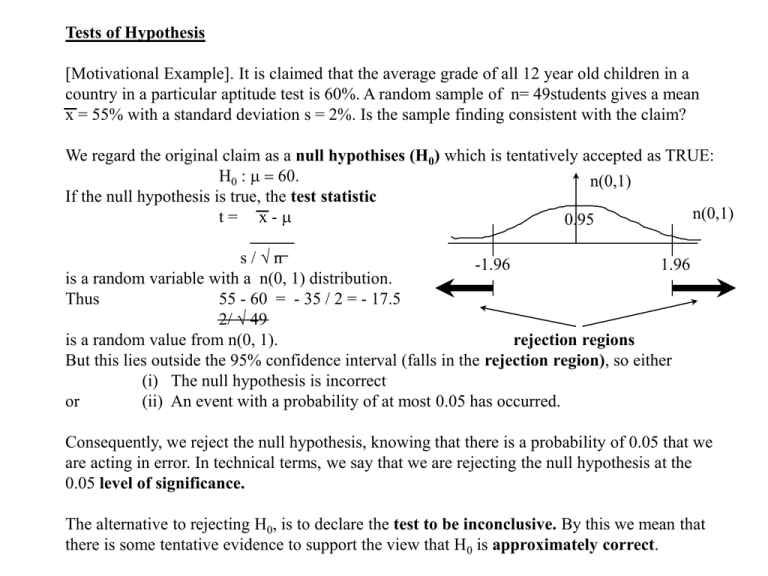
[Motivational Example]. It is claimed that the average grade of all 12 year old children in a
country in a particular aptitude test is 60%. A random sample of n= 49students gives a mean
x = 55% with a standard deviation s = 2%. Is the sample finding consistent with the claim?
We regard the original claim as a null hypothises (H0) which is tentatively accepted as TRUE:
H0 : m = 60.
n(0,1)
If the null hypothesis is true, the test statistic
n(0,1)
t= x-m
0.95
sn
-1.96
1.96
is a random variable with a n(0, 1) distribution.
Thus
55 - 60 = - 35 / 2 = - 17.5
2/  49
is a random value from n(0, 1).
rejection regions
But this lies outside the 95% confidence interval (falls in the rejection region), so either
(i) The null hypothesis is incorrect
or
(ii) An event with a probability of at most 0.05 has occurred.
Consequently, we reject the null hypothesis, knowing that there is a probability of 0.05 that we
are acting in error. In technical terms, we say that we are rejecting the null hypothesis at the
0.05 level of significance.
The alternative to rejecting H0, is to declare the test to be inconclusive. By this we mean that
there is some tentative evidence to support the view that H0 is approximately correct.
Modifications
Based on the propoerties of the normal , student t and other distributions, we can generalise
these ideas. If the sample size n < 25, we should use a tn-1 distribution, we can vary the level
of significance of the test and we can apply the tests to proportionate sampling
environments.
Example. 40% of a random sample of 1000 people in a country indicate satisfaction with
government policy. Test at the .01 level of significance if this consistent with the claim that
45% of the people support government policy?
Here,
H0: P = 0.45
p = 0.40,
n = 1000
so
 p (1-p) / n = 0.015 test statistic = (0.40 - 0.45) / 0.015 = - 3.33
99% critical value = 2.58
so H0 is rejected at the .01 level of significance.
One-Tailed Tests
If the null hypothesis is of the form H0 : P  0. then arbitrary large values of p are
acceptable, so that the rejection region for the test statistic lies in the left hand tail only.
Example. 40% of a random sample of 1000 people in a country indicate satisfaction with
government policy. Test at the .05 level of significance if this consistent with the claim that
at least 45% of the people support government policy?
n(0,1)
Here the critical value is -1.64, so the
0.95
the null hypothesis H0: P  0.
is rejected at the .05 level of
significance
-1.64
Rejection region
Testing Differences between Means
Suppose that
x 1 x2
…
xm is a random sample with mean x and standard deviation s1
drawn from a distribution with mean m1 and
y1 y2
…
yn is a random sample with mean y and standard deviation s1
drawn from a distribution with mean m2. Suppose that we wish to test the null hypothesis that
both samples are drawn from the same parent population (i.e.)
H0: m1 = m2.
The pooled estimate of the parent variance is
s 2 = { (m - 1) s12 + (n - 1) s22 } / ( m + n - 2)
and the variance of x - y, being the variance of the difference of two independent random
variables, is
s ’ 2 = s 2 / m + s 2 / n.
This allows us to construct the test statistic, which under H0 has a tm+n-2 distribution.
Example. A random sample of size m = 25 has mean x = 2.5 and standard deviation s1 = 2,
while a second sample of size n = 41 has mean y = 2.8 and standard deviation s2 = 1. Test at
the .05 level of significance if the means of the parent populations are identical.
Here
H0 : m1 = m2
x - y = - 0.3 and
s 2 = {24(4) + 38(1)} / 64 = 2.0313
so the test statistic is
- 0.3 /  .0    .0   = - 0.89
The .05 critical value for n(0, 1) is .96, so the test is inconclusive.
Paired Tests
If the sample values ( xi , yi ) are paired, such as the marks of students in two
examinations, then let
di = xi - yi be their differences and treat these
values as the elements of a sample to generate a test statistic for the hypothesis
H0: m1 = m2.
The test statistic
d / sd / n
has a tn-1 distribution if H0 is true.
Example. In a random sample of 100 students in a national examination their examination
mark in English is subtracted from their continuous assessment mark, giving a mean of 5
and a standard deviation of 2. Test at the .01 level of significance if the true mean mark for
both components is the same.
Here
n = 100, d = 5,
sd / n = 2/10 = 0.2
so the test statistic is 5 / 0.2 = 10.
the 0.1 critical value for a n(0, 1) distribution is 2.58, so H0 is rejected at the .01 level of
significance.
Tests for the Variance.
For normally distributed random variables, given
H0: s 2 = k, a constant, then
(n-1) s2 / k has a c 2n - 1 distribution.
Example. A random sample of size 30 drawn from a normal distribution has variance s2 = 5.
Test at the .05 level of significance if this is consistent with H0 : s 2 = 2 .
Test statistic = (29) 5 /2 = 72.5, while the .05 critical value for c 229 is 45.72,
so H0 is rejected at the .05 level of significance.
Chi-Square Test of Goodness of Fit
This can be used to test the hypothesis H0 that a set of observations is consistent with a given
probability distribution. We are given a set of categories and for each we record the observed
Oj nd expected Ej number of observations that fall in each category. Under H0,
the test statistic
S (Oj - Ej )2 / Ej
has a c 2n - 1 distribution, where n is the
number of categories.
Example.A pseudo random number generator is used to used to generate 40 random numbers
in the range 1 - 100. Test at the .05 level of significance if the results are consistent with the
hypothesis that the outcomes are randomly distributed.
Range
Observed Number
Expected Number
1-25
6
10
26 - 50
12
10
51 - 75
14
10
76 - 100 Total
8
40
10
40
Test statistic = (6-10)2/10 + (12-10)2/10 + (14-10)2/10 + (8-10)2/10 = 4.
The .05 critical value of c 23 = 7.81, so the test is inconclusive.
Chi-Square Contingency Test
To test that two random variables are statistically independent, a set of obsrvations can be
recorded in a table with m rows corresponding to categories for one random variable and
n columns for the other. Under H0, the expected number of observations for the cell in row i
and column j is the appropriate row total by the column total divided by the grand total.
Under H0, the test statistic
S (Oij - Eij )2 / Eij
has a c 2(m -1)(n-1) distribution.
Chi-Square Contingency Test - Example
In the following table, the
figures in brackets are the
expected values.
The test statistic is
Results
Honours
Pass
Fail
Totals
Maths
History
Geography
100 (50)
70 (67)
30 (83)
130 (225) 320 (300) 450 (375)
70 (25)
10 (33)
20 (42)
300
400
500
Totals
200
900
100
1200
S (Oij - Eij )2 / Eij = (100-50)2/ 50 + (70 - 67)2/ 67 + (30-83)2/ 83 + (130-225)2/ 225
+ (320-300)2/ 300 + (450-375)2/375 + (70-25)2/ 25 + (10-33)2/ 33 + (20-42)2/ 42
= 248.976
The .05 critical value for c 22 * 2 is 9.49 so H0 is rejected at the .05 level of significance.
In general the chi square tests tend to be very conservative vis-a-vis other tests of
hypothesis,
(i.e.) they tend to give inconclusive results.
A full explanation of the meaning of the term “degrees of freedom” is beyond the scope of
this course. In simplified terms, as the chi-square distribution is the sum of, say k, squares of
independent random variables, it is defined in a k-dimensional space. When we impose a
consraint of the type that the sum of observed and expected observations in a column are
equal or estimate a parameter of the parent distribution, we reduce the dimensionality of the
space by 1. In the case of the chi-square contingency table, with m rows and n columns, the
expected values in the final row and column are predetermined, so the number of degrees of
freedom of the test statistic is (m-1) (n-1).
Analysis of Variance
Analysis of Varianve (AOV) was originally devised within
the realm of agricultural statistics for testing the yields of 1
various crops under different nutrient regimes. Typically,
2
a field is divided into a regular array, in row and column
3
format, of small plots of a fixed size. The yield yi, j
within each plot is recorded.
y1, 1
y1, 2
y1, 3
y2, 1
y2, 2
y2, 3
y3, 1
y3, 2
y3, 3
y1, 4
y1, 5
If the field is of irregular width, different crops can be grown in each row and we can regard
the yields as replicated results for each crop in turn. If the field is rectangular, we can grow
different crops in each row and supply different nutrients in each column and so study the
interaction of two factors simultaneously. If the field is square, we can incorporate a third

factor. By replicating the sampling over many fields, very sophisticated interactions can be
studied.
One - Way Classification
Model:
where
yi, j = m +  i +
 i, j
,
 i ,j -> n (0, s)
m = overall mean
 i = effect of the ith factor
 i, j = error term.
Hypothesis:
H0:
 1 = 2 = …
=
m
Factor 1
2
y1, 1 y1, 2 y1, 3
y1, n1
y2, 1 y2,, 2 y2, 3 y1, n2
m ym, 1 ym, 2 ym, 3
ym, nm
y =   yi, j / n,
Overall mean
Totals
T1 =  y1, j
Means
y1. = T1 / n1
T2 =  y2, j
y2. = T2 / n2
Tm =  ym, j
ym. = Tm / nm
where n =  ni
Decomposition of Sums of Squares:
2
 ni (yi . - y )2
=
  (yi, j - y )
+   (yi, j - yi. )2
Total Variation (Q) = Between Factors (Q1) + Residual Variation (QE )
Under H0:
Q / (n-1) -> c
Q1 / ( m - 1 )
QE / ( n - m )
AOV Table: Variation
2
n - 1,
Q1 / (m - 1) -> c
2
m - 1,
QE / (n - m) -> c 2n - m
-> Fm - 1, n - m
D.F.
Sums of Squares
Mean Squares
Between
m -1
Q1=  ni(yi. - y )2 MS1 = Q1/(m - 1)
Residual
n-m
QE=   (yi, j - yi .)2 MSE = QE/(n - m)
Total
n -1
Q =   (yi, j. - y )2
Q /( n - 1)
F
MS1/ MSE
Two - Way Classification
Factor I
Factor II y1, 1 y1, 2 y1, 3
y1,
ym, 1 ym, 2 ym, 3
Means
y1.
n
ym, n
ym .
Means
y. 1 y. 2 y. 3
y .n
y
Decomposition of Sums of Squares:
  (yi, j - y )2 = n (yi . - y )2 + m  (y. j - y )2 +   (yi, j - yi . - y. j + y)2
Total
Between
Between
Residual
Variation
Rows
Columns
Variation
Model:
H0:
yi, j = m +
 i +  j+
All  i are equal and all
AOV Table: Variation
Between
Rows
Between
Columns
Residual
Total
D.F.
 i, j ,

i, j
-> n ( 0, s)
 j are equal
Sums of Squares
Mean Squares
F
m -1
Q1= n  (yi. - y )2
MS1 = Q1/(m - 1)
MS1/ MSE
n -1
Q2= m  (y.j - y )2
MS2 = Q2/(n - 1)
MS2/ MSE
(m-1)(n-1)
mn -1
QE=  (yi, j - yi . - y. j + y)2 MSE = QE/(m-1)(n-1)
Q = 
(yi, j. - y )2
Q /( mn - 1)
Two - Way AOV [Example]
Factor I
Factor II 1
2
3
4
Totals
Means
1
20
19
23
17
79
19.75
2
3
18
21
18
17
21
22
16
18
73
78
18.25 19.50
4
23
18
23
16
80
20.00
5 Totals Means
20
102 20.4
18
90 18.0
20
109 21.8
17
84 16.8
75
385
18.75
19.25
Variation d.f. S.S.
F
Rows
3 76.95 18.86**
Columns 4
8.50 1.57
Residual 12 16.30
Total
19 101.75
Note that many statistical packages, such as SPSS, are designed for analysing data that is
recorded with variables in columns and individual observations in the rows.Thus the AOV
data above would be written as a set of columns or rows, based on the concepts shown:
Variable
Factor 1
Factor 2
20 18 21 23 20 19 18 17 18 18 23 21 22 23 20 17 16 18 16 17
1 1 1 1 1 2 2 2 2 2 3 3 3 3 3 4 4 4 4 4
1 2 3 4 1 2 3 4 1 2 3 4 1 2 3 4 1 2 3 4
Normal Regression Model ( p independent variables) - AOV
p
Model:
y =  0 +   i x i+
1
SSR =  ( yi - y ) 2
SSE =  ( yi - yi ) 2
SST =  ( yj - y ) 2
 ,
-> n (0, s)
Source
d.f. S.S. M.S.
F
Regression p SSR MSR MSR/MSE
Error
n-p-1 SSE MSE
Total
n -1 SST
-
-
Latin Squares
We can incorporate a third source of variation in our
models by the use of latin squares. A latin square is a
design with exactly one instance of each “letter” in
each row and column.
Model:
yi, j = m +

i
+ 
j
+ 
l
+

i, j
A
B
C
D
B
D
A
C
C
A
D
B

,
i, j
D
C
B
A
-> n ( 0, s)
Latin Square Component
Column Effects
Row Effects
Decomposition of Sums of Squares (and degrees of freedom) :
  (yi, j - y )2 = n  (yi . - y )2 + n  (y. j - y )2 + n (y. l - y )2
+   (yi, j - yi . - y. j - yl + 2 y)2
Total
Between
Between
Latin Square
Residual
Variation
Rows
Columns
Variation
Variation
(n2 - 1)
(n - 1)
(n -1)
(n - 1)
(n - 1) (n - 2)
H0:
All
 i are equal, all

i
are equal and all 
i are
equal.
Experimental design is used heavily in management, educational and sociological
applications. Its popularity is based on the fact that the underlying normality conditions are
easy to justify, the concepts in the model are easy to understand and reliable software is
available.
Elementary Forecasting Methods
A Time Seties is a set of regular observations Zt taken over time. By the term spot estimate
we mean a forecast in a model that works under deterministic laws.
Exponential Smoothing.
This uses a recursively defined smoothed series St and a doubly smoothed series St [2] .
Exponential smoothing requires very little memory and has a single parameter  . For
commercial applications, the value  = 0.7 produces good results.
Filter:
St
= Zt + (1 -  ) St-1,

[ 0, 1]
= Zt + (1 - ) Zt-1 + (1 - )2 St-2
St[2] =
 St +
(1 -
) St-1[2]
Forecast: ZT+m = {2 ST - ST[2]} + {ST - ST[2]} m / (1 Example [  = 0.7]
Time t 1971
72
73
Zt
66
72 101
St
(66)
70.2 91.8
St[2]
(66)
68.9 84.9
Z1983 =
74 75
145 148
129.0 142.3
115.8 134.3
76
171
162.4
154.0
)
77
185
178.2
170.9
78
221
208.2
197.0
79
229
222.7
214.5
{2 (355.7) - 333} + {355.7 - 333} (2) (0.7) / (0.3) = 484.3
80
81
345 376
308.3 355.7
280.2 333.0
Moving Average Model.
If the time series contains a seasonal component over n “seasons”, the Moving Average
model can be used to generate deseasonalised forecasts.
t - n 1
Filter:
Mt
= 
i =t
Xi / n = Mt - 1 + { Zt - Zt - n } / n
t - n 1
Mt[2]
= 
Mt / n
i =t
Forecast: ZT + k= { 2 MT - MT[2] } + { MT - MT[2] } 2 k / ( n - 1)
Example.
Time t 1988
1989
Sp Su Au Wi Sp Su Au
ZT
5 8
5 13
7 10
6
MT
- 7.75 8.25 8.75 9.00
MT[2]
- - 8.44
1990
1991
Wi Sp Su Au Wi Sp Su Au Wi
15 10 13 11 17 12 15 14 20
9.50 10.25 11.00 12.25 12.75 13.25 13.75 14.50 15.25
8.88 9.38 9.94 10.75 11.56 12.31 13.00 13.56 14.19
The deseasonalised forecast for Sp 1992, which is 4 periods beyond the last observation, is
ZT+4 = { 2 15.25 - 14.19 } + { 15.25 - 14.19 } 2 (4) / 3 = 19.14
In simple multiplicative models we assume that the components are
Zt = T (trend) * S(seasonal factor) * R (residual term).
The following example demonstrates how to extricate these components from a series.
Time
t
Sp 1988
(1) Raw
(2) Four Month (3) Centered (4) Moving (5) Detrended (6) Deseasonalised (7) Residual
Data
Moving Total Moving Total Average
Data (1) / (4) Data (1)/(Seasonal) Series (6) / (4)
Zt =T*S*R
T*R
T
T
S*R
T*R
R
5
--
--
--
5.957
--
--
--
--
7.633
--
64
8.000
62.500
7.190
89.875
68
8.500
152.941
9.214
108.400
71
8.875
78.873
8.340
93.972
74
9.250
108.108
9.541
103.146
79
9.875
60.759
8.628
87.363
85
10.625
141.176
10.631
100.057
93
11.625
86.022
11.914
102.486
100
12.500
104.000
12.403
99.224
104
13.000
84.615
15.819
121.685
108
13.500
125.926
12.049
89.252
113
14.125
84.956
14.297
101.218
119
14.875
100.840
14.311
96.208
--
Su
8
31
Au
5
33
Wi
13
35
Sp 1989
7
Su
10
Au
6
36
38
41
Wi
15
44
Sp 1990
10
49
Su
13
Au
11
Wi
17
51
53
55
Sp 1991
12
58
Su
15
61
Au
14
Wi
20
---
---
---
20.133
--
---
---
---
14.175
--
--
The seasonal data is got by rearranging
column (5). The seasonal factors are then
reused in column (6)
Sp
1988
-1989 78.873
1990 86.022
Due to round-off errors in the arithmetic,
1991 84.956
it is necessary to readjust the means, so
Means 83.284
that they add up to 400 (instead of 396.905). Factors 83.933
The diagram illustrates the components
present in the data. In general when
analysing time series data, it is important
to remove these basic components before
proceeding with more detailed analysis.
Otherwise, these major components will
dwarf the more subtle component, and
will result in false readings.
The reduced forecasts are multiplied by
the appropriate trend and seasonal
components, at the end of the analysis.
Su
-108.108
104.000
100.840
104.316
105.129
Au
62.500
60.759
84.615
-69.291
69.831
Wi
152.941
141.176
125.926
-140.014
141.106
Raw Data
20
Trend
10
1988
1989
1990
1991
The forecasts that result from the models above, are referred to as “spot estimates”. This is
meant to convey the fact that sampling theory is not used in the analysis and so no
confidence intervals are possible. Spot estimates are unreliable and should only be used to
forecast a few time periods beyond the last observation in the time series.
Normal Linear Regression Model
In the model with one independent variable, we assume that the true relationship is
y = b0 + b1 x
and that our observations (x1, y1), (x2, y2), … , (xn, yn) is a random sample from the bivariate
parent distribution, so that
y= 0+ 1x+ ,
where  -> n( 0, s ).
If the sample statistics are calculated, as in the deterministic case, then  0,  1 and r are
unbiased estimates for the true values, b0, b1 and  , where r and  are the correlation
coefficients of the sample and parent distributions, respectively.
If
y=0+ 
1
x0 is the estimate for y given the value x0, then our estimate ofs
2
s2 = SSE / (n - 2) =  ( yi - yi )2 / (n - 2)
and
VAR [ y] = s2 { 1 + 1/n + (x0 - x ) 2 /  ( xi - x ) 2 }.
The standardised variable derived from y has a tn - 2 distribution, so confidence intervals for
the true value of y corresponding to x0 is
y0 + tn - 2 s
1 + 1/n + (x0 - x ) 2 /  ( xi - x ) 2 .
is
Example. Consider our previous regression example:
y = 23 / 7 + 24 / 35 x
xi
0
1
2
3
4
5
yi
3
5
4
5
6
7
yi
3.286 3.971 4.657 5.343 6.029 6.714
2
(yi - yi ) 0.082 1.059 0.432 0.118 0.001 0.082
=>
 ( yi - yi )2 = 1.774, s2 = 0.4435,
 (x - x )2 = 17,5,
x = 2.5,
i
Let
Then
f(x0) = t4, 0.9 s 1 + 1/n + (x0 - x )2 /
x0
0
1
2
3
f(x0)
2.282 2.104 2.009 2.009
y0 - f(x0) 1.004 1.867 2.648 3.334
y0 + f(x0) 5.568 6.075 6.666 7.352
The diagram shows the danger of extrapulation.
It is important in forecasting that the trend is
initially removed from the data so that the
slope of the regression line is kept as close to
zero as possble.
A description of the Box-Jenkins methodology
and Spectral Analysis, which are the preferred
techniques for forecasting commercial data, is
to be found in standard text books.
(6)
7.40
s
= 0.666,
t4, 0.95 = 2.776, t4, 0.95 (s) = 1.849
 (xi - x )2 .
95% Confidence
4
2.104
3.925
8.133
Interval when x=6
5
6
2.282 2.526
4.432 4.874
8.996 9.926
8
Y
6
4
2
X
6