Useful algorithms and statistical
methods in Genome data analysis
Ahmed Rebaï
Centre of Biotechnology of Sfax
ahmed.rebai@cbs.rnrt.tn
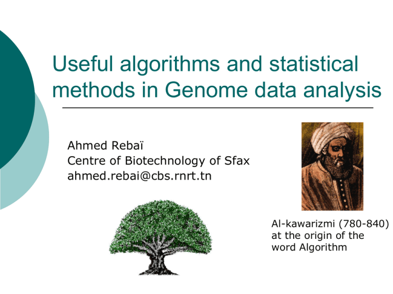
Al-kawarizmi (780-840)
at the origin of the
word Algorithm
Basic statistical concepts and
tools
Primer on:
Random variable
Random distribution
Statistical inference
Statistics


Statistics concerns the ‘optimal’
methods of analyzing data generated
from some chance mechanism
(random phenomena).
‘Optimal’ means appropriate choice
of what is to be computed from the
data to carry out statistical analysis
Random variables


A random variable is a numerical
quantity that in some experiment,
that involve some degree of
randomness, takes one value from
some ‘discrete’ set of possible values
The probability distribution is a set of
values that this random variable takes
together with their associated
probability
Three very important distributions!



The Binomial distribution: the number of
successes in n trials with two outcomes
(succes/failure) each, where proba. of sucess p is
the same for all trials and trials are independant
Pr(X=k)=n!/(n-k)!k! pk (1-p)n-k
Poisson distribution: the limiting form of the
binomial for large n and small p (rare events)
when np= is moderate
Pr(X=k)=e- k/ k!
Normal (Gaussian) distribution: arises in many
biological processes, limiting distribution of all
random variables for large n.
 1 ( x   )2 
1
f ( x) 
exp 

2
 2
2



Statistical Inference



Process of drawing conclusions about a
population on the basis of measurments
or observation on a sample of individuals
from the population
Frequentist inference: an approach
basedon a frequency (long-run) view of
probability with main tools: Tests,
likelihood (the probability of a set of
observations x giventhe value of some
set of parameters : L(x/))
Bayesian inference
Hypothesis testing





Significance testing: a procedure when applied
to a set of obs. results in a p-value relative to
some ‘null’ hypothesis
P-value: probability of observed data when the
null hypothesis is true, computed from the
distribution of the test statistic
Significance level: the level of probability at
which it is argued that the null hypothesis will
be rejected. Conventionnally set to 0.05.
False positive: reject nul hypothsis when it is
true (type I error)
False negative: accept null hypothesis when it
is false (type II error)
Bayesian inference

Approach based on Bayes’ theorem:





Obtain the likelihood L(x/)
Obtain the prior distrbution L() expressing
what is known about , before observing data
Apply Bayes’ theorrem to derive de the
posterior distribution L(/x) expresing what is
known about  after observing the data
Derive appropriate inference statement from
the posterior distribution: estimation,
probability of hypothesis
Prior distribution respresent the
investigators knowledge (belief) about the
parameters before seeing the data
Resampling techniques: Bootstrap





Used when we cannot know the exact
distribution of a parameter
sampling with replacement from the orignal
data to produce random samples of same
size n;
each bootstrap sample produce an
estimate of the parameter of interest.
Repeating the process a large number of
times provide information on the variability
of the estimator
Other techniques
 Jackknife: generates n samples each of size n-1
by omitting each member in turn from the data
Multivariate analysis
A primer on:
Discriminant analysis
Principal component analysis
Correspondance analysis
Exploratory Data Analysis (EDA)


Data analysis that emphasizes the use of
informal graphical porcedures not based on
prior assumptions about the structure of the
data or on formal models for the data
Data= smooth + rough where the smooth is
the underlying regulariry or pattern in the
data. The objective of EDA is to separate the
smooth from the rough with minimal use of
formal mathematics or statistics methods
Classification and clustering
Classification
Clustering
• known number of classes
• unknown number of classes
• based on a training set
• no prior knowledge
• used to classify future observations
• used to understand (explore) data
• Classification is a form of
supervised learning
• Clustering a form of unsupervised
learning
Classification

In classification you do
have a class label (o
and x), each defined
in terms of G1 and G2
values.
G1
*
*
*
* **
* * o
*
o o
o
o o
o
o
o
o

G2
You are trying to find a
model that splits the
data elements into
their existing classes
Supervised
Learning
G1

You then assume that
this model can be
used to assign new
data points x and y to
the right class
*
* o o
*
o
* **
o
o
o
* *
x?
*
o
o
o
y?
o
G2
Linear Discriminant Analysis




Proposed by Fisher (1936) for classifying an
obervation into one of two possible groups using
measurements x1,x2,…xp.
Seek a linear transformation of the variables
z=a1x1+a2x2+..apxp such that the separation
between the group means on the transformed scale
: a=S-1 (x1-x2) where x1 and x2 are mean vectors
of the two groups and S the pooled covariance
matrix of the two groups
Assign subject to group 1 if zi-zc<0 and to group 2
if zi-zc>0 where zc=(z1+z2)/2 is the group means
Subsets of variable most useful for discrimination
can be selected by regression procedures
Linear (LDA) and Quadratic (QDA)
discriminant analysis for gene prediction

Simple approach.


Training set (exons and non-exons)
Set of features (for internal exons)
donor/acceptor site recognizers
 octonucleotide preferences for coding region
 octonucleotide preferences for intron interiors
 on either side



Rule to be induced: linear (or quadratic)
combination of features.
Good accuracy in some circumstances
(programs: Zcurve, MZEF)
LDA and QDA in gene prediction
Principal Component Analysis



Introduced by Pearson (1901) and
Hotelling (1933) to describe the
variation in a set of multivariate data in
terms of a set of uncorrelated variables,
yi each of which is a linear combination
of the original variables (xi):
Yi= ai1x1+ai2x2+…aipxp where i=1..p
The new variables Yi are derived in
decreasing order of importance; they
are called ‘principal components’
Principal Component Analysis
How to avoid correlated features?
Correlations  covariance matrix is non-diagonal
Solution: diagonalize it, then use transformation
that makes it diagonal to de-correlate features
Columns of Z are eigenvectors and diagonal
elements of  are eigenvalues
Y  ZT X; CX Z( i )  i Z( i ) ; CX Z  ZΛ
CY  ZT CX Z  ZT ZΛ  Λ
Properties of PCA
Small i  small variance  data change little in
direction Yi
PCA minimizes C matrix reconstruction errors
Zi vectors for large i are sufficient because
vectors for small eigenvalues will have very small
contribution to the covariance matrix.
The adequacy of representation by the two first
components is measured by
% explanation= (1 + 2) / i
True covariance matrices are usually not known,
estimated from data.
Use of PCA


PCA is useful for: finding new, more
informative, uncorrelated features;
reducing dimensionality: reject low
variance features,..
Analysis of expression data
Correspondance analysis (Benzecri, 1973)





For uncovering and understanding the structure and
pattern in data in contingency tables.
Involves finding coordinate values which represent
the row and column categories in some optimal way
Coordinates are obtained from the Singular value
decomposition (SVD) of a matrix E which elements
are: eij=(pij- pi. p.j)/(pi. p.j)1/2
E=UDV’, U eigenvectors of EE’, V eigenvectors of
E’E and D a diagonal matrix with k singular values
(²k eigenvalues of either EE’ or E’E)
The adequacy of representation by the two first
coordinates is measured by
% inertia= (²1+²2)/²k
Properties of CA


allows consideration of dummy variables
and observations (called ‘illustrative
variables or observations’), as additional
variables (or observations) which do not
contribute to the construction of the
factorial space, but can be displayed on this
factorial space.
With such a representation it is possible to
determine the proximity between
observations and variables and the
illustrative variables and observations.
Example: analysis of codon usage and
gene expression in E. coli (McInerny, 1997)
A gene can be represented by a 59dimensional vector (universal code)
A genome consists of hundreds (thousands) of
these genes
Variation in the variables (RSCU values) might
be governed by only a small number of
factors
For each gene and each codon i calculate
RCSUi=# observed cordon i/#expected codon i
Do Correspondance analysis on RSCU
Plot of the two most important axes after correspondence analysis
of RSCU values from the E. coli genome.
Lowly-expressed
genes
Highly
expressed
genes
Recently
acquired genes
Other Methods



Factor analysis: ‘explain’ correlations between a
set of p variables in terms of a smaller number
k<p of unobservable latent variables (factors):
x=Af+u , S=AA’+D where D is a diagonal
matrix and A is a matrix of factor loadings
Multidimensional Scaling: construct a lowdimentional geometrical representation of a
distance matrix
Cluster analysis:a set of methods for contructing
sensible and informative classification of an
initially unclassified set of data using the variable
values observed on each individual (hierarchical
clustering, K-means clustering, ..)
Datamining or KDD




Process of seeking interesting and
valuable information within large
databases
Extension and adaptation of standard
EDA procedures
Confluence of ideas from statistics,
EDA, machine learning, pattern
recognition, database technology, etc.
Emphasis is more on algorithms rather
than mathematical or statistical models
Famous Algorithms in
Bioinformatics
A primer on:
HMM
EM
Gibbs sampling (MCMC)
Hidden Markov Models
Historical overview




Introduced in 1960-70 to model
sequences of observations
Observations are discrete (character
from some alphabet) or continious
(signal frequency)
First applied in speech recognition
since 1970
Applied to biological sequences since
1992: multiple alignment, profile,
gene prediction, fold recognition, ..
Hidden Markov Model (HMM)



Can be viewed as an abstract machine
with k hidden states.
Each state has its own probability
distribution, and the machine switches
between states according to this
probability distribution.
At each step, the machine makes 2
decisions:
 What state should it move to next?
 What symbol from its alphabet should it
emit?
Why “Hidden”?


Observers can see the emitted symbols
of an HMM but has no ability to know
which state the HMM is currently in.
Thus, the goal is to infer the most likely
states of an HMM basing on some given
sequence of emitted symbols.
HMM Parameters
Σ: set of all possible emission characters.
Ex.: Σ = {H, T} for coin tossing
Σ = {1, 2, 3, 4, 5, 6} for dice tossing
Q: set of hidden states {q1, q2, .., qn},
each emitting symbols from Σ.
A = (akl): a |Q| x |Q| matrix of probability
of changing from state k to state l.
E = (ek(b)): a |Q| x |Σ| matrix of
probability of emitting symbol b during a
step in which the HMM is in state k.
The fair bet casino problem





The game is to flip coins, which results in only
two possible outcomes: Head or Tail.
Suppose that the dealer uses both Fair and
Biased coins.
The Fair coin will give Heads and Tails with
same probability of ½.
The Biased coin will give Heads with prob. of
¾.
Thus, we define the probabilities:
 P(H|F) = P(T|F) = ½
 P(H|B) = ¾, P(T|B) = ¼
 The crooked dealer changes between Fair
and Biased coins with probability 10%
The Fair Bet Casino Problem


Input: A sequence of x = x1x2x3…xn
of coin tosses made by two possible
coins (F or B).
Output: A sequence π = π1 π2 π3… πn,
with each πi being either F or B
indicating that xi is the result of
tossing the Fair or Biased coin
respectively.
HMM for ‘Fair Bet Casino’

The Fair Bet Casino can be defined in
HMM terms as follows:
Σ = {0, 1} (0 for Tails and 1 Heads)
Q = {F,B} – F for Fair & B for Biased
coin.
aFF = aBB = 0.9
aFB = aBF = 0.1
eF(0) = ½
eF(1) = ½
eB(0) = ¼
eB(1) = ¾
HMM for Fair Bet Casino
Visualization of the Transition probabilities A
Biased
Fair
Biased
aBB = 0.9 aFB = 0.1
Fair
aBF = 0.1 aFF = 0.9
Visualization of the Emission Probabilities E
Biased
Fair
Tails(0)
eB(0) = ¼ eF(0) = ½
Heads(1)
eB(1) = ¾ eF(1) = ½
HMM for Fair Bet Casino
HMM model for the Fair Bet Casino Problem
Hidden Paths


A path π = π1… πn in the HMM is defined as a
sequence of states.
Consider path π = FFFBBBBBFFF and sequence x
= 01011101001
Probability of xi was emitted from state πi
x
π
0 1
=
0 1
1 1
0
1 0
0 1
F F F B B B B B F F F
P(xi|πi)
½ ½ ½ ¾ ¾ ¾ ¾ ¾ ½ ½ ½
P(πi-1  πi)
½
9/
10
9/
10
1/
10
9/
10
9/
10
9/
10
9/
10
1/
10
9/
10
9/
10
Transition probability from state πi-1 to state πi
P(x|π) Calculation

P(x|π): Probability that sequence x was
generated by the path π, given
the model M.
n
P(x|π) = P(π0→ π1) . Π P(xi| πi).P(πi →
πi+1)
i=1
=a
n
π0, π1
.Πe
i=1
πi
(xi) . a
πi, πi+1
Forward-Backward Algorithm
Given: a sequence of coin tosses generated by an
HMM.
Goal: find the probability that the dealer was using
a biased coin at a particular time.
 The probability that the dealer used a biased coin
at any moment i is as follows:
P(x, πi = k)
fk(i) . bk(i)
P(πi = k|x) = _______________ = ______________
P(x)
P(x)
Forward-Backward Algorithm
 fk,i (forward probability) is the probability of emitting

the prefix x1…xi and reaching the state π = k.
The recurrence for the forward algorithm is:
fk,i = ek(xi) . Σ fk,i-1 . alk
lЄQ


Backward probability bk,i ≡ the probability of being
in state πi = k and emitting the suffix xi+1…xn.
The backward algorithm’s recurrence:
bk,i = Σ el(xi+1) . bl,i+1 . Akl
lЄQ
HMM Parameter Estimation





So far, we have assumed that the transition and
emission probabilities are known.
However, in most HMM applications, the
probabilities are not known and hard to estimate.
Let Θ be a vector combining the unknown
transition and emission probabilities.
Given training sequences x1,…,xm, let P(x|Θ) be
the max. prob. of x given the assignment of
param.’s Θ.
m
Then our goal is to find
maxΘ Π P(xi|Θ)
j=1
The Expectation Maximization
(EM) algorithm
Dempster and Laird (1977)
EM Algorithm in statistics



An algorithm producing a sequence of
parameter estimates that converge to
MLE. Have two steps:
E-step: calculate de expected value of the
likelihood conditionnal on the data and the
current estimates of the parameters
E(L(x/i))
M-step: maximize the likeliood to give
updated parameter estimates increasing L


The two steps are alternated until convergence
Needs a first ‘guess’ estimate to start
The EM Algorithm for motif detection
• This
algorithm is used to identify conserved areas in
unaligned sequences.
• Assume that a set of sequences is expected to have a
common sequence pattern.
• An initial guess is made as to location and size of the
site of interest in each of the sequences and these parts
are loosely aligned.
• This alignment provides an estimate of base or aa
composition of each column in the site.
EM algorithm in motif finding



The EM algorithm consists of the two steps,
which are repeated consecutively:
Step 1: the Expectation step, the columnby-column composition of the site is used to
estimate the probability of finding the site at
any position in each of the sequences. These
probabilities are used to provide new
information as to expected base or aa
distribution for each column in the site.
Step 2: the Maximization step, the new
counts for bases or aa for each position in
the site found in the step 1 are substituted
for the previous set.
Expectation Maximization (EM) Algorithm
OOOOOOOOXXXXOOOOOOOO
OOOOOOOOXXXXOOOOOOOO
o o o o o o o o o o o o o o o o o o o o o o o o
OOOOOOOOXXXXOOOOOOOO
OOOOOOOOXXXXOOOOOOOO
IIII
IIIIIIII
Columns defined by a preliminary
alignment of the sequences provide
initial estimates of frequencies of aa
in each motif column
IIIIIII
Columns not in motif provide
background frequencies
Bases
Background
Site column
1
Site column
2
……
G
0.27
0.4
0.1
……
C
0.25
0.4
0.1
……
A
0.25
0.2
0.1
……
T
0.23
0.2
0.7
……
Total
1.00
1.00
1.00
……
EM Algorithm in motif finding
XXXXOOOOOOOOOOOOOOOO
XXXX
A
IIII
IIIIIIIIIIIIIIII
OXXXXOOOOOOOOOOOOOOO
XXXX
B
IIII
I
IIIIIIIIIIIIIII
Use previous estimates of aa
or nucleotide frequencies for
each column in the motif to
calculate probability of motif
in this position, and multiply
by……..
X
…background frequencies in the
remaining positions.
The resulting score gives the likelihood that the motif
matches positions A, B or other in seq 1. Repeat for
all other positions and find most likely locator. Then
repeat for the remaining seq’s.
EM Algorithm 1st expectation step :
calculations
• Assume that the seq1 is 100 bases long and the length of the site
is 20 bases.
• Suppose that the site starts in the column 1 and the first two
positions are A and T.
• The site will end at the position 20 and positions 21 and 22 do not
belong to the site. Assume that these two positions are A and T also.
• The Probability of this location of the site in seq1 is given by
Psite1,seq1 = 0.2 (for A in position 1) x 0.7 (for T in position 2) x Ps
(for the next 18 positions in site) x 0.25 (for A in first flanking
position) x 0.23 (for T in second flanking position x Ps (for the next
78 flanking positions).
EM Algorithm 1st expectation step :
calculations (continued)



The same procedure is applied for calculation of
probabilities for Psite2,seq1 to Psite78, seq1,
thus providing a comparative set of probabilities
for the site location.
The probability of the best location in seq1, say
at site k, is the ratio of the site probability at k
divided by the sum of all the other site
probabilities.
Then the procedure repeated for all other
sequences.
EM Algorithm 2nd optimisation step:
calculations
• The site probabilities for each seq calculated at the 1st step are
then used to create a new table of expected values for base counts
for each of the site positions using the site probabilities as weights.
• Suppose that P (site 1 in seq 1) = Psite1,seq1 / (Psite1,seq1 + Psite2,seq1 +
…+ Psite78,seq1 ) = 0.01 and P (site 2 in seq 1) = 0.02.
• Then this values are added to the previous table as shown in the
table below.
Bases
Backgroun
Site column
Site column
……
d
1
2
G
0.27 + …
0.4 + …
0.1 + …
……
C
0.25 + …
0.4 + …
0.1 + …
……
A
0.25 + …
0.2 + 0.01
0.1 + …
……
T
0.23 + …
0.2 + …
0.7 + 0.02
……
Total/
weighted
1.00
1.00
1.00
……
EM Algorithm 2nd optimisation step:
calculations
* This procedure is repeated for every other
possible first columns in seq1 and then the
process continues for all other sequences
resulting in a new version of the table.
* The expectation and maximization steps
are repeated until the estimates of base
frequencies do not change
Gibbs sampling
Gibbs sampling and the Motif Finding
Problem
Given a list of t sequences each of length n,
Find the best pattern of length l that
appears in each of the t sequences.
Let s denote the set of starting positions
s = (s1,...,st) for l-mers in our t
sequences. Then the substrings
corresponding to these starting positions
will form a t x l alignment matrix and a
4 x l profile matrix* which we will call P.
Let Prob(a|P) be defined as the probability
that an l-mer a was created by Profile P
Scoring Strings with a Profile
Given a profile: P =
A
1/2
7/8
3/8
0
1/8
0
C
1/8
0
1/2
5/8
3/8
0
T
1/8
1/8
0
0
1/4
7/8
G
1/4
0
1/8
3/8
1/4
1/8
The probability of the consensus string:
Prob(aaacct|P) = 1/2 x 7/8 x 3/8 x 5/8 x 3/8 x 7/8 = .033646
Probability of a different string:
Prob(atacag|P) = 1/2 x 1/8 x 3/8 x 5/8 x 1/8 x 7/8 = .001602
Gibbs Sampling
1) Choose uniformly at random starting positions
s = (s1,...,st) and form the set of l-tuples
associated with these starting positions.
2) Randomly choose one of the t sequences.
3) Create a profile P from the other t -1 seq.
4) For each position in the removed sequence,
calculate the probability that the l-mer starting at
that position was generated by P.
5) Choose a new starting position for the
removed sequence at random based on the
probabilities calculated in step 4.
6) Repeat steps 2-5 until no improvement on the
starting positions can be made.
An Example of Gibbs Sampling: motifs
finding in DNA sequences
Input:
t = 5 sequences where L = 8
1. GTAAACAATATTTATAGC
2. AAAATTTACCTCGCAAGG
3. CCGTACTGTCAAGCGTGG
4. TGAGTAAACGACGTCCCA
5. TACTTAACACCCTGTCAA
Start the Gibbs Smapling
1) Randomly choose starting positions,
S=(s1,s2,s3,s4) in the 4 sequences and
figure out what they correspond to:
S1=7
GTAAACAATATTTATAGC
S2=11 AAAATTTACCTTAGAAGG
S3=9
CCGTACTGTCAAGCGTGG
S4=4
TGAGTAAACGACGTCCCA
S5=1
TACTTAACACCCTGTCAA
2) Choose one of the sequences at random:
Sequence 2: AAAATTTACCTTAGAAGG
An Example of Gibbs Sampling
3) Create profile from remaining
subsequences:
1
A
A
T
A
T
T
T
A
3
T
C
A
A
G
C
G
T
4
G
T
A
A
A
C
G
A
5
T
A
C
T
T
A
A
C
A
1/4
2/4
2/4
3/4
1/4
1/4
1/4
2/4
C
0
1/4
1/4
0
0
2/4
0
1/4
T
2/4
1/4
1/4
1/4
2/4
1/4
1/4
1/4
G
1/4
0
0
0
1/4
0
3/4
0
Consensu
s
String
T
A
A
A
T
C
G
A
An Example of Gibbs Sampling
4) Calculate the prob(a|P) for every
possible 8-mer in the removed
sequence:
Strings Highlighted in Red
prob(a|P)
AAAATTTACCTTAGAAGG
AAAATTTACCTTAGAAGG
AAAATTTACCTTAGAAGG
AAAATTTACCTTAGAAGG
AAAATTTACCTTAGAAGG
AAAATTTACCTTAGAAGG
AAAATTTACCTTAGAAGG
AAAATTTACCTTAGAAGG
AAAATTTACCTTAGAAGG
AAAATTTACCTTAGAAGG
AAAATTTACCTTAGAAGG
.000732
.000122
0
0
0
0
0
.000183
0
0
0
An Example of Gibbs Sampling
5) Create a distribution of probabilities, and
based on this distribution, randomly select a
new starting position.
a) Create a ratio by dividing each probability
by the lowest probability:
Starting Position 1: prob( AAAATTTA | P ) = .000732 / .000122 = 6
Starting Position 2: prob( AAATTTAC | P ) = .000122 / .000122 = 1
Starting Position 8: prob( ACCTTAGA | P ) = .000183 / .000122 = 1.5
Ratio = 6 : 1 : 1.5
An Example of Gibbs Sampling
b) Create a distribution so that the most
probable start position is chosen at random
with the highest probability:
P(selecting starting position 1):
.706
P(selecting starting position 2):
.118
P(selecting starting position 8):
.176
An Example of Gibbs Sampling
Assume we select the substring with the highest
probability – then we are left with the following new
substrings and starting positions.
S1=7
GTAAACAATATTTATAGC
S2=1
AAAATTTACCTCGCAAGG
S3=9
CCGTACTGTCAAGCGTGG
S4=5
TGAGTAATCGACGTCCCA
S5=1
TACTTCACACCCTGTCAA
6) We iterate the procedure again with the
above starting positions until we cannot
improve the score any more.
Problems with Gibbs Sampling
1.
2.
Gibbs Sampling often converges to local
optimum motifs instead of global
optimum motifs.
Gibbs Sampling can be very complicated
when applied to samples with unequal
distributions of nucleotides
Useful books: general
Usefull book: technical
Usefull books: statistical