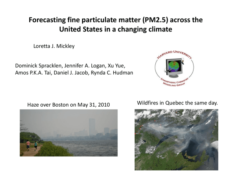
Forecasting fine particulate matter (PM2.5) across the
United States in a changing climate
Loretta J. Mickley
Dominick Spracklen, Jennifer A. Logan, Xu Yue,
Amos P.K.A. Tai, Daniel J. Jacob, Rynda C. Hudman
Haze over Boston on May 31, 2010
Wildfires in Quebec the same day.
Atmospheric chemistry examines the mix of gases and particles in the atmosphere:
• Chemical reactions
• Distributions in the atmosphere
• Effects on climate and health
• Effects of climate on smog
Lifetimes in atmospheric chemistry
Centuries: SF6, some CFCs
Pollution over Hong Kong
Decades: most greenhouse gases:
CO2, N2O, . . .
9-10 years: CH4 (methane,
precursor to ozone and
greenhouse gas)
Days-weeks: O3 (ozone),
particulate matter (PM, aka
aerosols)
Seconds: OH, NO
Air pollution over Hong Kong reached dangerous
levels one of every eight days in 2009
2
Surface ozone and particulate matter are harmful
to human health.
Number of people living in areas that exceed the national
ambient air quality standards (NAAQS) in 2008.
Calculated with standard of
0.075 ppm. Proposed new
standards will push more
areas into non-attainment.
Bars on barplot will change with changing emissions of ozone precursors.
Climate change could also change the size of these bars, by changing the dayto-day weather.
SO2 -- sulfur dioxide
NOx -- nitrogen oxides
Life cycle of particulate
matter (PM, aerosols)
precursor gases
ultra-fine
(<0.01 mm)
nucleation
Soup of
chemical
reactions
VOCs -- volatile
organic compounds
NH3 -- ammonia
fine
(0.01-1 mm)
. . coagulation
.
. . .
condensation
cloud
(1-100 mm)
cycling
coarse
scavenging
(1-10 mm)
SO2
NOx
SO2
NOx
VOCs
combustion
volcanoes
NOx
VOCs
VOCs
VOCs
VOCs
NH3
NOx
NOx
agriculture
biosphere
wildfires
combustion
soil dust
sea salt 4
Climate change affects many
processes.
Life cycle of particulate matter (PM, aerosols)
precursor gases
ultra-fine
(<0.01 mm)
nucleation
Soup of
chemical
reactions
faster reactions
SO2
NOx
SO2
NOx
VOCs
combustion
volcanoes
fine
(0.01-1 mm)
. . coagulation
.
. . .
condensation
Warmer temperatures could
increase some emissions.
NOx
VOCs
VOCs
cycling
coarse
scavenging
(1-10 mm)
VOCs
VOCs
NH3
cloud
(1-100 mm)
NOx
NOx
agriculture
biosphere
wildfires
combustion
soil dust
sea salt 5
Transport also important!
Life cycle of particulate matter (PM, aerosols)
precursor gases
ultra-fine
(<0.01 mm)
nucleation
Soup of
chemical
reactions
NOx
SO2
NOx
VOCs
combustion
volcanoes
. . coagulation
.
. . .
condensation
evaporation
Warmer temperatures push
equilibrium toward gas phase.
faster reactions
SO2
fine
(0.01-1 mm)
NOx
VOCs
VOCs
cycling
coarse
scavenging
(1-10 mm)
VOCs
VOCs
NH3
cloud
(1-100 mm)
NOx
NOx
agriculture
biosphere
wildfires
combustion
soil dust
sea salt 6
Coming climate change will likely affect PM2.5 concentrations.
Models disagree on the sign and the magnitude of the impacts
Racherla and Adams, 2006
Response of sulfate PM2.5 at
the surface to 2000-2050
climate change.
• These model results are
computationally expensive.
A2
mg
m-3
• How well do models capture
variability in present-day
PM2.5?
Pye et al., 2009
We need a simple tool that will allow
AQ managers to readily calculate the
climate penalty for PM2.5 air quality
across a range of models and scenarios.
A1
mg m-3
7
Effects of wildfires on air quality in cities in Western US
 Hayman fire, June 8-22, 2002
 56,000 ha burned
 30 miles from Denver and Colorado Springs
Worst ever air quality in Denver
June 8, 2002
PM10 = 40 μg/m3
PM2.5 = 10 μg/m3
June 9, 2002 PM10 = 372 μg/m3
PM2.5 = 200 μg/m3
Standard = 35 µg/m3
Colorado Dept. of Public Health and Environment
Vedal et al., 2006
Fires are increasing in North America
obs temperature
area burned
5 yr means
1960
Area burned in Canada has
increased since the 1960s,
correlated with temperature
increase.
Gillett et al., 2004
2000
Increased fire frequency over the
western U.S. since 1970,
related to warmer temperatures
and earlier snow melt.
1970
2000
Westerling et al., 2007
Two constellations of studies
1. Sensitivity of PM2.5 to changing meteorology in
the East.
2. Sensitivity of wildfires to changing climate in the
West and the consequences for PM2.5.
First, a few slides on chemistry + climate models.
Basic working of climate models
All climate models depend on basic physics to describe motions and
thermodynamics of the atmosphere:
E.g., vertical structure of pressure is described by hydrostatic equation
P( z )  P( z  dz )   a gdz

dP
  a g
dz
Climate models also depend on parameterizations for
many processes.
E.g., microphysics of cloud droplet formation,
vegetation processes.
Input
Tilt of earth,
geography,
greenhouse
gas content
Climate model
Physics +
Parameterized
processes
Output
Weather +
Climate
11
Simulations of future climate depend on the path
of socio-economic development.
Global mean surface temperature anomalies
Different scenarios
follow different socioeconomic paths for
developed and
developing countries.
A2 = heavy fossil fuel
B1 = alternative fuels
A1B = mix of fossil +
alternative fuels
IPCC 2007
IPCC AR4 models show increasing temperatures across North
America by 2100 in A1B scenario.
Change in surface temperatures in 2100, relative to present-day.
Results for precipitation changes are not so clear.
IPCC, 2007
How 3-D chemistry models work.
emissions
transport
dilution
chemistry
particulate matter (PM)
and ozone pollution
population
GEOS-Chem chemical transport model:
Global 3-D model describes the transport and
chemical evolution of atmospheric pollutants
winds
Meteorology from
a climate model
Emissions + chemistry
calculated within box
Winds carry
pollutants to
other boxes.
14
Two constellations of studies
1. Sensitivity of PM2.5 to changing meteorology in
the East.
2. Sensitivity of wildfires to changing climate in the
West and the consequences for PM2.5.
Surface ozone levels are sensitive to cold-front passage.
Are particles also sensitive to cold-front passage?
Leibensperger et al., 2008
Meteorology affects surface concentrations of PM2.5.
Observed
correlations of PM2.5
with meteorological
variables.
1998-2008
meteorology + EPAAQS observations
Multiple linear regression coefficients for total PM2.5 on
meteorological variables. Units: μg m-3 D-1 (p-value < 0.05)
Increases in total PM2.5 on
a stagnant day vs. a nonstagnant day.
Mean PM2.5 is 2.6 μg m-3
greater on a stagnant day
Tai et al. 2010
17
2000-2050 climate change leads to increases in annual mean PM2.5
across much of the Eastern US.
We used Principal Component
Analysis to define the main
meteorological modes driving
PM2.5 variability over the US.
Change in annual mean PM2.5 concentrations
in 2050s relative to present-day
0.15
0.10
0.05
0.00
-0.05
-0.10
-0.15
mg m-3
Models show increased
duration of stagnation in the
East, with corresponding
increases in annual mean
PM2.5.
This approach could provide a
useful tool to assess climate
penalty on PM2.5.
We use observed relationships
+ climate models, no chemistry
models.
Tai et al., ms.
How do we predict fires in a future climate?
We don’t have a good mechanistic approach for modeling wildfires.
Relationship between observed
meteorology + area burned
1970
+
Future
meteorology
2000
Future area
burned
Predictions of area burned are made for large
eco-regions for the fire season
RMF
ERM
PNW
NMS
CCS
DSW
In each region, identify the
meteorological variables that
best predict area burned using
stepwise linear regression.
We find that the most important predictors for wildfires in the West are
temperature, relative humidity, and precipitation.
Ecoregions are aggregates of those in
Bailey et al. (1994)
Regression matches observed area burned,
except for California coastal shrub
Data
Fit
Fit depends on relative humidity the previous summer
Spracklen et al., 2009; Yue et al., ms.
GISS GCM meteorological output used to project future area burned,
emissions and changes in air quality
GISS climate model
1950 Spin-up 2000
Area Burned
Regressions
changing greenhouse gases (A1B scenario)
2025
2050
2075
2100
archive met fields from
climate model
GEOS-CHEM
Predict Area
Burned
Calculate
emissions
Global chemistry model
50% increase in biomass consumption by wildfires
over the western United States for 2045-2054,
relative to present-day.
Effect of future fires in a future climate on organic carbon
in the western U.S.
May-October change in OC
Change in organic carbon
(OC) by 2050s, relative to
present-day (5 year mean)
Organic carbon particles increase by 40% by 2050.
Black carbon increases by 20%.
For OC, most of increase is from fire emissions, some is from higher biogenic
emissions in a warmer climate.
Spracklen et al., JGR, 2009
Results shown so far were driven by one climate model. But models
show large variation in response to changing greenhouse gases.
Temp
Results from IPCC AR4
ensemble of climate
models: warmer, drier,
less humid.
Precip
Changes in meteorology
by 2050s, relative to
present-day, for JJA
RMF
Rel Humidity
PNW
NMS
CCS
DSW
ERM
PNW, Pacific Northwest
CCS, California Coastal Shrub
DSW, Desert Southwest
NMS, Nevada /Semi-desert
RMF, Rocky Mountain Forest
ERM, East Rockies/ Plains.
Yue et al., ms.
1986-2000
2051-2065
+40%
1986
2065
Obs
Wildfires in western US
are predicted to increase
by ~60% by 2050s.
+20%
Area burned (ha)
Median of models
spread of models
doubling
+60%
The GCMs cannot match year to year
variability, but match the mean area
burned fairly well in present-day.
RMF
+70%
ERM
PNW
NMS
CCS
DSW
+60%
Yue et al., ms.
Forest
Ratio of 2050s area burned / present-day area burned
Forest
Ratio of 2050s / present-day
Median GCM results show an increase in
area burned in all regions.
median
Median changes:
40-70% increase in
forested regions
60% increase in grasslands
Doubling in Southwest
RMF
ERM
PNW
NMS
CCS
DSW
Yue et al., ms.
Organic particles increase in future atmosphere over the
western U.S. in summer, especially during extreme events.
Change in OC in ~2050s,
relative to present-day
Cumulative probability of daily mean
concentrations of organic particles
2050s
doubling
Presentday
Rocky Mountains
April-October.
Yue et al., ms.
How do we improve fire predictions in S. California?
The largest fires in CA are associated with Santa Ana events.
Fire plumes (Oct. 2007)
Composite Santa Ana winds
Need finely resolved wind fields to
capture Santa Ana in meteorological
record.
Hughes and Hall (2010)
Area burned
Improving predictions of area burned
in Southern California.
Fire data from a suite of sources.
Surface pressure anomalies
Parameterize area burned as function of:
• Temperature
• Relative humidity
• Precipitation
• Large-scale pressure differences
Divide up southern California into 3
smaller ecoregions.
Yue et al., ms.
Seasonality of fires in Southern California
Fire regions
South-West Cal.
area
num. fires
Central Western Cal.
Largest area burned in SW California.
October peak associated with the Santa
Ana winds, which are underestimated by
large scale models as they lack the
detailed topography: need large-scale
approach
Sierra Nevada
New parameterization predicts yearly variability and
seasonality in south west California
Southwest CA
R2=0.64
Seasonality
Area burned in ~2050 / Present-day
Area burned in Southern
California increases 20-100% by
2050s relative to present-day.
R
P
South west
California
R
Central
California
R
P
Two approaches used in each
ecoregion.
Sierra Nevada
Yue et al., ms.
Conclusions
Models show increased duration of stagnation in future atmosphere, with
corresponding increases in annual mean PM2.5.
Wildfire activity in the West can be predicted with meteorological variables.
Area burned by wildfires may double in some regions in the western US by 2050s.
By 2050s, mean summertime organic carbon particles could increase 40-70%, with
doubling during extreme events.
Future regional predictions for meteorology in A1B 2100
atmosphere show large variation across North America.
Percent change in 2100 precipitation relative to present-day
Annual
DJF
JJA
Number of models showing increasing precipitation
most
models
few
models
IPCC 2007