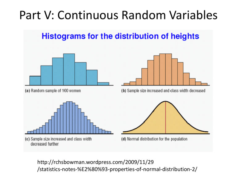
Part V: Continuous Random Variables
http://rchsbowman.wordpress.com/2009/11/29
/statistics-notes-%E2%80%93-properties-of-normal-distribution-2/
Chapter 23: Probability Density Functions
http://divisbyzero.com/2009/12/02
/an-applet-illustrating-a-continuous-nowhere-differentiable-function//
Comparison of Discrete vs. Continuous
(Examples)
Discrete
Continuous
Counting: defects, hits, die Lifetimes, waiting times,
values, coin heads/tails,
height, weight, length,
people, card
proportions, areas,
arrangements, trials until
volumes, physical
success, etc.
quantities, etc.
Comparison of mass vs. density
Mass (probability
mass function, PMF)
0 ≤ pX(x) ≤ 1
Density (probability density
function, PDF)
0 ≤ fX(x)
∞
𝑝𝑋 𝑥 = 1
𝑥
𝑓𝑋 𝑥 𝑑𝑥 = 1
−∞
P(0 ≤ X ≤ 2) = P(X = 0)
𝑃
0
≤
𝑋
≤
2
=
+ P(X = 1) + P(X = 2)
P(X ≤ 3) ≠ P(X < 3)
when P(X = 3) ≠ 0
2
𝑓𝑋 𝑥 𝑑𝑥
0
P(X ≤ 3) = P(X < 3)
since P(X = 3) = 0 always
Example 1 (class)
Let x be a continuous random variable with
density:
1
𝑓𝑋 𝑥 = 24 2𝑥 + 3 1 ≤ 𝑥 ≤ 4
0
𝑒𝑙𝑠𝑒
a) What is P(0 ≤ X ≤ 3)?
b) Determine the CDF.
c) Graph the density.
d) Graph the CDF.
e) Using the CDF, calculate
P(0 ≤ X ≤ 3), P(2.5 ≤ X ≤ 3)
Example 1 (cont.)
1
f(x)
0.8
0.6
0.4
0.2
0
0
1
2
3
4
5 1
x
0.8
F(x)
-1
0.6
0.4
0.2
0
-1
0
1
2
x
3
4
5
Example 2
Let X be a continuous function with CDF as
follows
0
𝑥<0
𝐹𝑋 𝑥 = 𝑥 2 0 ≤ 𝑥 ≤ 1
1
1<𝑥
What is the density?
Comparison of CDFs
Function
Discrete
Continuous
𝐹𝑋 𝑎 = 𝑃 𝑋 ≤ 𝑎
𝐹𝑋 𝑎 = 𝑃 𝑋 ≤ 𝑎
=
=
𝑃(𝑋 = 𝑎)
𝑥≤𝑎
graph
graph
Step function with
jumps of the same
size as the mass
Range: 0 ≤ X ≤ 1
𝑎
𝑓𝑋 𝑥 𝑑𝑥
−∞
continuous
Range: 0 ≤ X ≤ 1
Example 3
Suppose a random variable X has a density given
by:
4
𝑘𝑥
0
<
𝑥
<
4
𝑓𝑋 𝑥 =
0
𝑒𝑙𝑠𝑒
Find the constant k so that this function is a
valid density.
Example 4
Suppose a random variable X has the following
density:
1
0<𝑥<1
2
𝑓𝑋 𝑥 = 1
1≤𝑥≤4
6
0
𝑒𝑙𝑠𝑒
a) Find the CDF.
b) Graph the density.
c) Graph the CDF.
-1
1
0.8
0.6
0.4
0.2
0
0
1
2
3
4
5
x
1
0.8
F(x)
f(x)
Example 4 (cont.)
0.6
0.4
0.2
0
-1
0
1
2
x
3
4
5
Mixed R.V. – CDF
Let X denote a number selected at random from
the interval (0,4), and let Y = min(X,3).
Obtain the CDF of the random variable Y.
1
0.8
0.6
0.4
0.2
0
-1
0
1
2
3
4
Chapter 24: Joint Densities
http://www.alexfb.com/cgi-bin/twiki/view/PtPhysics/WebHome
Probability for two continuous r.v.
http://tutorial.math.lamar.edu/Classes/CalcIII/DoubleIntegrals.aspx
Example 1 (class)
A man invites his fiancée to a fine hotel for a
Sunday brunch. They decide to meet in the
lobby of the hotel between 11:30 am and 12
noon. If they arrive a random times during this
period, what is the probability that they will
meet within 10 minutes? (Hint: do this
geometrically)
Example: FPF (Cont)
40
30
20
10
0
-10
0
-10
10
20
30
40
Example 2 (class)
Consider two electrical components, A and B, with
respective lifetimes X and Y. Assume that a joint PDF of
X and Y is
fX,Y(x,y) = 10e-(2x+5y), x, y > 0
and fX,Y(x,y) = 0 otherwise.
a) Verify that this is a legitimate density.
b) What is the probability that A lasts less than 2 and B
lasts less than 3?
c) Determine the joint CDF.
d) Determine the probability that both components are
functioning at time t.
e) Determine the probability that A is the first to fail.
f) Determine the probability that B is the first to fail.
Example 2d
t
t
Example 2e
y=x
Example 2e
y=x
Example 3
Suppose a random variables X and Y have a joint
density given by:
𝑘𝑥𝑦 0 < 𝑥, 𝑦 < 2
𝑓𝑋,𝑌 𝑥, 𝑦 =
0
𝑒𝑙𝑠𝑒
Find the constant k so that this function is a
valid density.
Example 4 (class)
Suppose a random variables X and Y have a joint
density given by:
𝑥 + 𝑦 0 < 𝑥, 𝑦 < 1
𝑓𝑋,𝑌 𝑥, 𝑦 =
0
𝑒𝑙𝑠𝑒
a) Verify that this is a valid joint density.
b) Find the joint CDF.
c) From the joint CDF calculated in a), determine
the density (which should be what is given
above).
Example: Marginal density (class)
A bank operates both a drive-up facility and a walk-up
window. On a randomly selected day, let X = the
proportion of time that the drive-up facility is in use
(at least one customer is being served or waiting to
be served) and Y = the proportion of time that the
walk-up window is in use. The joint PDF is
6
2
(x

y
) 0  x  1,0  y  1

fX,Y (x,y)   5

0
else
a) What is fX(x)?
b) What is fY(y)?
Example: Marginal density (homework)
A nut company markets cans of deluxe mixed nuts
containing almonds, cashews and peanuts. Suppose the
net weight of each can is exactly 1 lb, but the weight
contribution of each type of nut is random. Because the
three weights sum to 1, a joint probability model for
any two gives all necessary information about the
weight of the third type. Let X = the weight of almonds
in a selected can and Y = the weight of cashews. The
joint PDF is
24xy 0  x  1,0  y  1,x  y  1
fX ,Y (x,y)  
else
 0
a) What is fX(x)?
b) What is fY(y)?
Chapter 25: Independent
Why’s everything got to be so intense with me?
I’m trying to handle all this unpredictability
In all probability
-- Long Shot, sung by Kelly Clarkson, from the album All
I ever Wanted; song written by Katy Perry, Glen Ballard,
Matt Thiessen
Example: Independent R.V.’s
A bank operates both a drive-up facility and a walk-up
window. On a randomly selected day, let X = the
proportion of time that the drive-up facility is in use
(at least one customer is being served or waiting to
be served) and Y = the proportion of time that the
walk-up window is in use. The joint PDF is
6
2
 (x  y ) 0  x  1,0  y  1
fX,Y (x,y)   5

0
else
6
2
3 6 2
𝑓𝑋 𝑥 = 𝑥 + , 𝑓𝑌 𝑦 = + 𝑦
5
5
5 5
Are X and Y independent?
Example: Independence
Consider two electrical components, A and B,
with respective lifetimes X and Y with
marginal shown densities below which are
independent of each other.
fX(x) = 2e-2x, x > 0, fY(y) = 5e-5y, y > 0
and fX(x) = fY(y) = 0 otherwise.
What is fX,Y(x,y)?
Example: Independent R.V.’s (homework)
A nut company markets cans of deluxe mixed nuts
containing almonds, cashews and peanuts. Suppose
the net weight of each can is exactly 1 lb, but the
weight contribution of each type of nut is random.
Because the three weights sum to 1, a joint
probability model for any two gives all necessary
information about the weight of the third type. Let
X = the weight of almonds in a selected can and Y =
the weight of cashews. The joint PDF is
24xy 0  x  1,0  y  1,x  y  1
fX ,Y (x,y)  
else
 0
Are X and Y independent?
Chapter 26: Conditional Distributions
Q : What is conditional probability?
A : maybe, maybe not.
http://www.goodreads.com/book/show/4914583-f-in-exams
Example: Conditional PDF (class)
Suppose a random variables X and Y have a joint
density given by:
𝑥 + 𝑦 0 < 𝑥, 𝑦 < 1
𝑓𝑋,𝑌 𝑥, 𝑦 =
0
𝑒𝑙𝑠𝑒
a) Calculate the conditional density of X when Y = y
where 0 < y < 1.
b) Verify that this function is a density.
c) What is the conditional probability that X is
between -1 and 0.5 when we know that Y = 0.6.
d) Are X and Y independent? (Show using
conditional densities.)
Chapter 27: Expected values
http://www.qualitydigest.com/inside/quality-insider-article
/problems-skewness-and-kurtosis-part-one.html#
Comparison of Expected Values
Discrete
Continuous
∞
𝔼 𝑋 =
𝑥𝑝𝑋 (𝑥)
𝑥
𝔼 𝑋 =
𝑥𝑓𝑋 𝑥 𝑑𝑥
−∞
Example: Expected Value (class)
What is the expected value in each of the following
situations:
a) The following is the
density of the
magnitude X of a
dynamic load on a
bridge (in newtons)
1 3
  x 0x2
fX (x)   8 8
 0
else
b) The train to Chicago
leaves Lafayette at a
random time between
8 am and 8:30 am. Let
X be the departure
time.
 2 8  x  8.5
fX (x)  
else
0
Chapter 28: Functions, Variance
http://quantivity.wordpress.com/2011/05/02/empirical-distribution-minimum-variance/
Comparison of Functions, Variances
Discrete
Function
(general)
Continuous
𝔼 𝑔(𝑋)
𝔼 𝑔(𝑋)
=
=
∞
𝑔(𝑥)𝑝𝑋 (𝑥)
−∞
𝑥
Function
2 =
𝔼
𝑋
(X2)
𝑔(𝑥)𝑓𝑋 𝑥 𝑑𝑥
∞
𝑥 2 𝑝𝑋 (𝑥) 𝔼 𝑋 2 =
𝑥 2 𝑓𝑋 𝑥 𝑑𝑥
−∞
𝑥
Variance Var(X) = 𝔼(X2) – (𝔼(X))2 Var(X) = 𝔼(X2) – (𝔼(X))2
SD
𝜎𝑋 =
𝑉𝑎𝑟(𝑋)
𝜎𝑋 =
𝑉𝑎𝑟(𝑋)
Example: Expected Value - function
(class)
What is 𝔼(X2) in each of the following situations:
a) The following is the
density of the
magnitude X of a
dynamic load on a
bridge (in newtons)
1 3
  x 0x2
fX (x)   8 8
 0
else
b) The train to Chicago
leaves Lafayette at a
random time between
8 am and 8:30 am. Let
X be the departure
time.
 2 8  x  8.5
fX (x)  
else
0
Example: Variance (class)
What is the variance in each of the following
situations:
a) The following is the
density of the
magnitude X of a
dynamic load on a
bridge (in newtons)
1 3
  x 0x2
fX (x)   8 8
 0
else
b) The train to Chicago
leaves Lafayette at a
random time between
8 am and 8:30 am. Let
X be the departure
time.
 2 8  x  8.5
fX (x)  
else
0
Friendly Facts about Continuous
Random Variables - 1
• Theorem 28.18: Expected value of a linear
sum of two or more continuous random
variables:
𝔼(a1X1 + … + anXn) = a1𝔼(X1) + … + an𝔼(Xn)
• Theorem 28.19: Expected value of the product
of functions of independent continuous
random variables:
𝔼(g(X)h(Y)) = 𝔼(g(X))𝔼(h(Y))
Friendly Facts about Continuous
Random Variables - 2
• Theorem 28.21: Variances of a linear sum of
two or more independent continuous random
variables:
Var(a1X1 + … + anXn) =𝑎12 Var(X1) + … + 𝑎𝑛2 Var(Xn)
• Corollary 28.22: Variance of a linear function
of continuous random variables:
Var(aX + b) = a2Var(X)
Chapter 29: Summary and Review
http://www.ux1.eiu.edu/~cfadd/1150/14Thermo/work.html
Example: percentile
Let x be a continuous random variable with
density:
1
𝑓𝑋 𝑥 = 24 2𝑥 + 3 1 ≤ 𝑥 ≤ 4
0
𝑒𝑙𝑠𝑒
0
𝑥<1
1 2
𝐹𝑋 𝑥 =
𝑥 + 3𝑥 − 4 1 ≤ 𝑥 ≤ 4
24
1
4<𝑥
a) What is the 99th percentile?
b) What is the median?