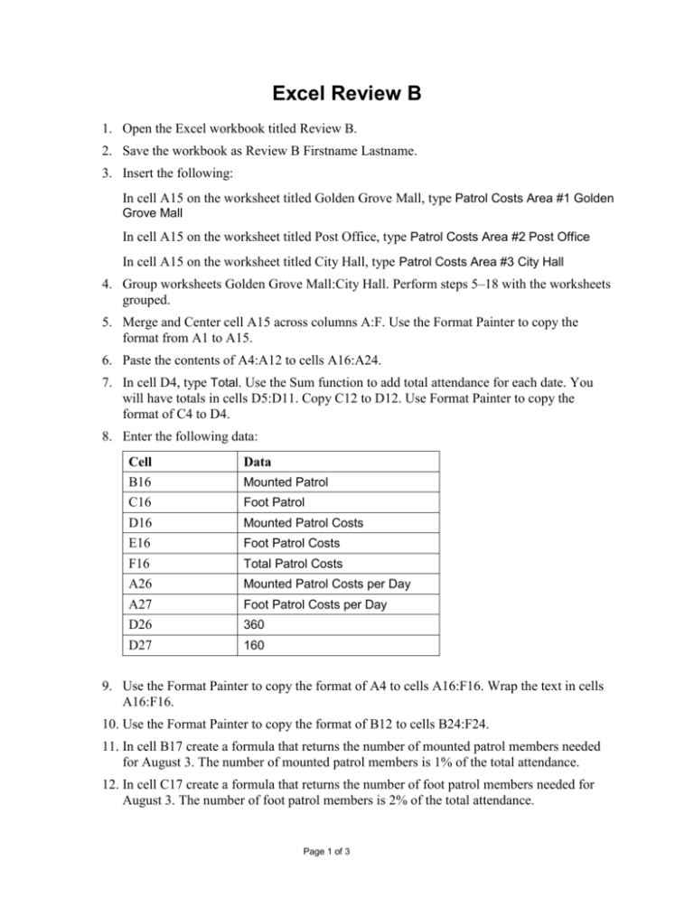
Excel Review B
1. Open the Excel workbook titled Review B.
2. Save the workbook as Review B Firstname Lastname.
3. Insert the following:
In cell A15 on the worksheet titled Golden Grove Mall, type Patrol Costs Area #1 Golden
Grove Mall
In cell A15 on the worksheet titled Post Office, type Patrol Costs Area #2 Post Office
In cell A15 on the worksheet titled City Hall, type Patrol Costs Area #3 City Hall
4. Group worksheets Golden Grove Mall:City Hall. Perform steps 5–18 with the worksheets
grouped.
5. Merge and Center cell A15 across columns A:F. Use the Format Painter to copy the
format from A1 to A15.
6. Paste the contents of A4:A12 to cells A16:A24.
7. In cell D4, type Total. Use the Sum function to add total attendance for each date. You
will have totals in cells D5:D11. Copy C12 to D12. Use Format Painter to copy the
format of C4 to D4.
8. Enter the following data:
Cell
B16
C16
D16
E16
F16
A26
A27
D26
D27
Data
Mounted Patrol
Foot Patrol
Mounted Patrol Costs
Foot Patrol Costs
Total Patrol Costs
Mounted Patrol Costs per Day
Foot Patrol Costs per Day
360
160
9. Use the Format Painter to copy the format of A4 to cells A16:F16. Wrap the text in cells
A16:F16.
10. Use the Format Painter to copy the format of B12 to cells B24:F24.
11. In cell B17 create a formula that returns the number of mounted patrol members needed
for August 3. The number of mounted patrol members is 1% of the total attendance.
12. In cell C17 create a formula that returns the number of foot patrol members needed for
August 3. The number of foot patrol members is 2% of the total attendance.
Page 1 of 3
13. Use the fill handle to copy B17:C17 to B23:C23. Remove all decimals in cells B17:C23.
14. Create a formula in cell D17 that returns the cost of the Mounted Patrol for August 3. Use
the fill handle to copy the formula to cells D18:D23.
15. Create a formula in cell E17 that returns the cost of the Foot Patrol for August 3. Use the
fill handle to copy the formula to cells E18:E23.
16. Use a function in cell F17 to display the total patrol costs for August 3. Copy the function
to cells F18:F23.
17. Use a function to display the totals in cells B24:F24.
18. Format D17:F24 with Comma style. Format D26:D27 with Accounting style.
19. Insert a new worksheet. Move it to the left of the Golden Grove Mall worksheet. Rename
the new worksheet Patrol Cost Summary
20. Enter the following:
Cell
A1
A2
B3
C3
D3
A4
A5
A6
A7
Data
Summer Fair and Arts Festival
Patrol Costs August 3-9
Mounted Patrol Costs
Foot Patrol Costs
Total Patrol Costs
Golden Grove Mall
Post Office
City Hall
Total
21. Apply the following formats:
Cell
Format
A1:A2
Cambria, 14 point,
Font color – Orange, Accent 6,
Darker 25%, Bold
Merge and Center A:D
B3:D3
Calibri, 11 point, Font color –
Orange, Accent 6, Darker 25%,
Italic, Bold, Center, Middle Align
A4:A7
Calibri, 12 point, bold
22. AutoFit column A. Wrap the text in cells B3:D3.
23. Create formulas in cells B4:C6 that return the corresponding totals from the
corresponding worksheets.
Page 2 of 3
24. Use the Sum function in cells D4:D6 to total the mounted and foot patrol costs for each
location. AutoFit column D.
25. Use the Sum function in cells B7:D7 to display the total mounted patrol costs and the
total foot patrol costs. Format B7:D7 with a Top and Double Bottom Border.
26. Format B4:D7 with the Accounting style.
27. Create a footer for each worksheet with the following information:
Left side: file name
Center: Date
Right side: worksheet name
28. Save your workbook. Check your work against the answer key which is in your review
folder on your computer.
When Both Review A and Review B are completed:
 Have Jennifer evaluate both Review A and B when they are completed. Be sure to have
your homework checklist ready so she can mark the points received.
 Copy both Review A and Review B to your Review folder inside your Excel homework
folder on W.
 Print Review A only and attach it to your checklist.
 Turn your checklist in with Review A attached to the wooden box next to the printer in
Cloud 109.
Page 3 of 3