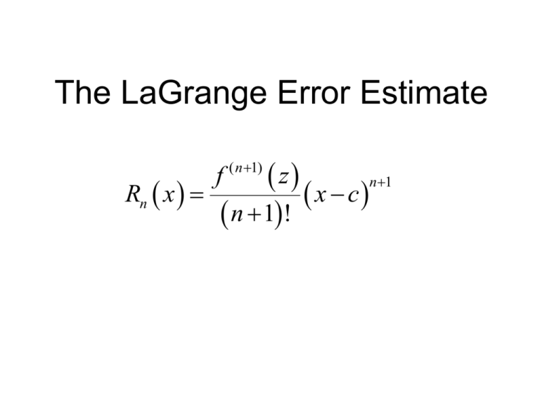
The LaGrange Error Estimate
Rn  x  
 z  x  c n1
 
 n  1!
f
( n 1)
THEOREM 9.19
TAYLOR’S THEOREM
If a function f is differentiable through order n + 1 in an interval I containing c, then,
for each x in I, there exists z between x and c such that
f (c)
f ( x)  f (c)  f (c)( x  c) 
( x  c) 2 
2!
Where
f ( n1) ( z )
Rn ( x) 
( x  c)n1
(n  1)!
.
f ( n ) (c )

( x  c) n  Rn ( x)
n!
Pn  x  is the nth degree polynomial centered at c used to estimate f  x 
at some fixed value of x.
Pn  x   f  c   f '  c  ( x  c ) 
f " c 
2
 x  c
2

f "'  c 
3!
x  c
3
 ... 
f (n)  c 
n!
x  c
n
Rn  x  is the difference between the function and the polynomial
at some fixed value of x.
Rn  x   f  x   Pn  x 
Fix x in I  x  c  , let t act as a variable in place of c and
n 1

x  t 

let g  t   f  x    Pn  t   Rn  x 
n 1

 x  c  

f "t 
f "'  t 
2
3
g  t   f  x    f  t   f '  t  x  t  
x

t

x

t
 
  
2
3!


f  n 1  t 
 n  1!
x  t
n 1

f  n t 
n!
x  t 
n

 x  t   Rn  x 
n 1
 x  c  
n 1

f "t 
f "'  t 
2
3
g  t   f  x    f  t   f '  t  x  t  
x

t

x

t
 
  
2
3!


t 
n 1
x  t 
 n  1!
f
 n 1
f
 n
t 
n!
x  t 

 x  t   Rn  x 
n 1
 x  c  
n 1
n
A couple of observations:
If we let t  x
g  x  0
If we let t  c
g c  0
Since g  x   g  c  , Rolle's Theorem guarantees
that for some value of t (lets call it z ), g '( z )  0.
So let's look at the derivative of g (t ) with respect to t.
n 1

f "t 
f "'  t 
f  n 1  t 
f  n t 
x  t   

d
d 
2
3
n 1
n
g  t    f  x    f  t   f '  t  x  t  

x t 
 x  t   ... 
x t 
 x  t   Rn  x 
n 1 
dt
dt 
2
3!
n  1!
n!

x

c

 




g '  t   0   f '  t   f " t  ( x  t )  f '  t  1 
f
 4
t 
3!
(x  t) 
f  n 1  t 
 n !
3
f "'  t 
3!
( x  t )n 
3 x  t   1  ...
2
f (n) t 
 n !
f  n  t 
 n  1!
f "'  t 
2
(x  t)
n 1

( x  t )2 
f ( n 1)  t 
 n  1!
f "t 
2
 n  1 x  t 
 x  t   1 

 n  1 Rn  x 
n 1
 x  c  
n
 n  x  t   1 
n 1
 2  x  t   1 
1
n2
 1 
f "'  t 
0   f '  t   f " t  ( x  t )  f ' t  1 
( x  t )2 
g ' t  
2
f  4  t 
3!
f
 n 1
(x  t) 
t 
 n !
3
f "'  t 
( x  t )n 
3!
 3 x  t   1 
2
f  n  t 
 n  1!
(x  t)
n 1

f "t 
2
f ( n 1)  t 
 n  1!
 2  x  t   1 
 n  1 x  t 
 x  t   1 
n 1

 n  x  t   1   n  1 Rn  x 
n 1
n
!
 
 x  c  
f (n) t 
n
1
n2
 1 
This telescoping effect leaves us with...
n
 f  n 1  t 
x  t   1 

n
g ' t    

( x  t )   n  1 Rn  x 
n 1
n
!



 x  c  
g ' t   
f  n 1  t 
x  t
( x  t )n   n  1 Rn  x 
n 1
 n !
 x  c
n
Recall that Rolle's theorem applies so
for some t  z between x and c, g '  z   0
g ' z   
f  n 1  z 
 x  z
( x  z )   n  1 Rn  x 
n 1
 n !
 x  c
n
n
0
g ' z   
f  n 1  z 
 x  z
( x  z )   n  1 Rn  x 
n 1
 n !
 x  c
n
n
x  z
 n  1 Rn  x 
n 1
 x  c
f  n 1  z 
n
 x  z
Rn  x 
n 1
 x  c

 n !
f  n 1  z 
n
Rn  x 
Rn  x  
f  n 1  z 
 n  1 n !

 x  c
 x  c
n 1
n 1
( x  z )n
 n  1 n !
1


0
( x  z )n
f  n 1  z 
 n  1 n !
f  n 1  z 
 n  1!
 x  c
n 1
Q.E.D.
quod erat demonstrandum- which was to be demonstrated
Consider the function
12
5 x
f  x 
 x 3
6


2 
n 0 

The Taylor series for f centered at x = 3 is
n
We could use the fourth degree polynomial to estimate f(2).
 x 3
 x 3
 x 3
 x 3
P4  x   6  6 

6

6

6







 2 
 2 
 2 
 2 
2
3
 23
 23
 23
 2 3
P4  2   6  6 

6

6

6







 2 
 2 
 2 
 2 
2
P4  2   6  3 
3 3 3
 
2 4 8
 4.125
f  2  4
Error = f  2   P4  2 
 0.125
3
4
4
We had the advantage of having a very basic function to evaluate at x = 2. What if
the function were not so easy to evaluate? We may not know the actual value of
the function at x = 2. Could we have any confidence in our estimate using this
polynomial?
The LaGrange Error Estimate
f  x   Pn  x   Rn  x  
f  2   P4  2   R4  x  
4  4.125  0.125 
f n 1  z 
 n  1!
f  5  z 
5!
f  5  z 
5!
 x  c
 2  3
5
 2  3
5
n 1



max f n 1  z 
 n  1!
max f  5  z 
5!
max f  5  z 
5!
 x  c
23
5
 2  3
5
n 1
We will need the maximum of the absolute value of the fifth derivative of our function.
We will be looking for this maximum in the interval between the center of the
polynomial and the value of x we are using for our approximation.
f  x 
12
5 x
f  5  x  
1440
5  x 
6
5
What is the maximum value of f    x  
1440
5  x 
6
 
on the interval 2,3
We could use a Graphing Calculator, look for critical numbers by setting the 6th
derivative equal to zero, or recognize that the 6th derivative is always positive
therefore the max of the 5th derivative occurs at the right endpoint.
The maximum will occur at x = 3
The maximum is 22.5
4  4.125  0.125 
f  5  z 
5!
 2  3
5

max f  5  z 
5!
 2  3
5

22.5 5
1  0.1875
5!
The series we used to estimate f(2) was P4  2   6  3 
Did you notice the series was alternating?
3 3 3
 
2 4 8
The error of an alternating series can be estimated by evaluating the first
neglected term.
3
 0.1875
16
Remember this is not the actual error (or remainder ). Instead it
bounds the error. In other words we know the remainder (error) must
be less than or possibly equal to 0.1875.
Example 7: Determining the Accuracy of the Approximation
x3
The third Maclaurin polynomial for sin x is given by P3 ( x)  x 
.
3!
Use Taylor’s Theorem to approximate sin(0.1) by P3 (0.1) and determine the
accuracy of the approximation.
P3 (0.1)   0.1 
Rn  x  
R3  0.1 
 0.1
3!
f  n 1  z 
 n  1!
f
4
 z
4!
3

1
1
599


 0.0998
10 6000 6000
 x  c
 0.1  0  
4
0  z  0.1
f  x   sin( x)
f '  x   cos  x 
f "  x    sin  x 
n 1
 x    cos  x 
4
f    x   sin  x 
f
max f 
4
4!
 z
 0.1  0 
3
4
What is the maximum value sin x could be?
1
4
Error   0.1  0.00000416666
4!
Example 8: Approximating a Value to a Desired Accuracy
Determine the degree of the Taylor polynomial Pn(x) expanded about c = 1 that should
be used to approximate ln(1.2) so that the error is less than 0.001.
f  x   ln x
1
f ' x 
x
1
f " x    2
x
f  3  x  
Error 
nn  312
2
x3
max f  n 1  z 
 n  1!
 x  c
n 1
 0.001
1  z  1.2
max
max
max
f  2ff1  zzz
2 1
1.2

1
1.2

1



1.2

1


1

1
!
3

1
!




 2  1!
 3111
3111
11
21 62 1 43 2
62 1 1.2
3

1
1  .2
 0.02
1.2
11
.2.2 0.0004
0.00266666

1.2

246 2
 3 2111!!1!
6
x4
We meet the error condition with n  3 so we need a third degree polynomial.
f  4  x  
1
2
2
3
 x  1   x  1
2
3!
1
2
2
3
P3 1.2   1.2  1  1.2  1  1.2  1  0.1826666666...
2
3!
P3  x    x  1 
ln 1.2  0.1823215568
The error is indeed less than 0.001
Even though we know Rn  x  exists, it may be impossible or impractical to find Rn  x  .
Example 8) Find the accuracy of the fourth Maclaurin polynomial for e0.1 .
One interpretation of the question would be to determine the actual error.
To do this, we will find f  0.1 and P3  0.1 and subract. Rn  0.1  f  0.1  Pn  0.1 .
From a calculator, we can determine f  0.1  0.904837418 Please note that this is just an estimate.
What is the fourth Maclaurin polynomial for e-0.1 ?
f  x   ex
f  0  1
f '  x   ex
f '  0  1
f " x   e x
f " 0  1
f "'  x   e x
f "'  0  1
f  4  x   e x
f  4  0   1
Pn  x   f  c   f '  c  x  c  
f " c 
2!
 x  c
P3  0.1  f  0   f '  0  0.1  0  
2
f " 0
2!

f "'  c 
3!
 x  c
 0.1  0 
3
2


f "'  0 
3!

f  n  c 
n!
 x  c
 0.1  0 
3
n
P3  0.1  f  0   f '  0  0.1  0  
P3  0.1  1   .1 
f " 0
2!
 0.1  0  
2
f "'  0 
3!
 0.1  0 
1
1
2
3

0.1


0.1
 
   0.90483333...
2!
3!
From the calculator, we got f  0.1  0.904837418
Rn  0.1  f  0.1  Pn  0.1
R3  0.1  0.904837418  0.90483333...  0.000004085
This would be the "exact" error.
3
The LaGrange Error Bound
Let's look at the graph of f  4  x   e x for  0.1  x  0.
0.1
We know that Rn  x  
f  n 1  z 
Rn  x  
 n  1!
z
 x  c 
max f  n 1  z 
 n  1!
n 1
xc
0
but how do we find z? What if we find z?
n 1
for  0.1  z  0
0.1
Rn  x  
max f  n 1  z 
 n  1!
R3  0.1 
z
xc
0
n 1
for  0.1  z  0
1
4
0.1  0  0.000004166666...
4!
R3  0.1  0.000004085
Here is another approach to the problem.
P3  0.1  1   .1 
1
1
2
3

0.1


0.1
 
 
2!
3!
P3  0.1  1   0.1 
1
1
2
3
0.1

 
 0.1
2!
3!
Since the series is alternating, the error is ...
f
R 3  -0.1 
 4
 x  e
f  4  0 
4!
f  4  0   1
x
 0.1  0 
Error  the next term
4

0.000004166666...


Example 9) Lef f be a function given by f  x   cos  2 x   and let P  x  be the third-degree Taylor Polynomial
6

1
1
1
about f at x  0. Use the Lagrange error bound to show that f    P   
.
3
3
100
 
 
Rn  x  
max f  n 1  z 
 n  1!
xc
n 1
for x  z  c
We will need the fourth derivative if our polynomial is a third degree polynomial.
n 1
max f  4  z  1
1
R3  x  
0
for 0  z 
3
3
 4 !


f  x   cos  2 x  
6



f '  x   2sin  2 x  
6



f '"  x   8sin  2 x  
6



f "  x   4 cos  2 x  
6



f  4  x   16 cos  2 x  
6

Let assume calculators are not permitted.
4
max f  4  z  1
1
R3  x  
 0 for 0  z 
3
3
 4 !
What is the MAX f  4  x  ?


f  4  x   16 cos  2 x  
6

4
2
16
2
16 1
1



R3  x  

 4 ! 3  2481  381 243 100
If calculators are permitted, graph f  4  x  .


f  4  x   16 cos  2 x  
6

0
1
3
What is the MAX f  4  x  ?
 3


max f  4  x   16 cos  2  0     16 

6
2



Rn  x  
max f  n 1  z 
 n  1!
xc
n 1
for 0  z 
1
3
 3
max f  4   x   16 

2


 3
16 

8 3
2  1 n 1


Rn  x  
 2481
 4 ! 3

3
 381

4
243

2
1

243
100
third
Example 10) Let f be a function having derivatives for all orders at all real numbers. The fourth-degree Taylor
5
20
2
3
polynomial for f about x  2 is given by: P  x   9  4  x  2    x  2    x  2  . The
3
7
 4
fourth derivative for f satisfies the inequality the f  x   25 for all x in the interval  2, 0 . Find
the Lagrange error bound for the approximation to f  1.6 
R3  x  
max f  4  z 
R3  x  
 4 !
1.6  2
4
for -2  z  1.6
25
4
25
4
1.6  2 
.4 

 4 !
24
R3  x   0.02666...
What is the MAX f  4  x  ?
 0.02666...