Calculus Formulas First derivative of a function f(x) =0 gives critical
advertisement
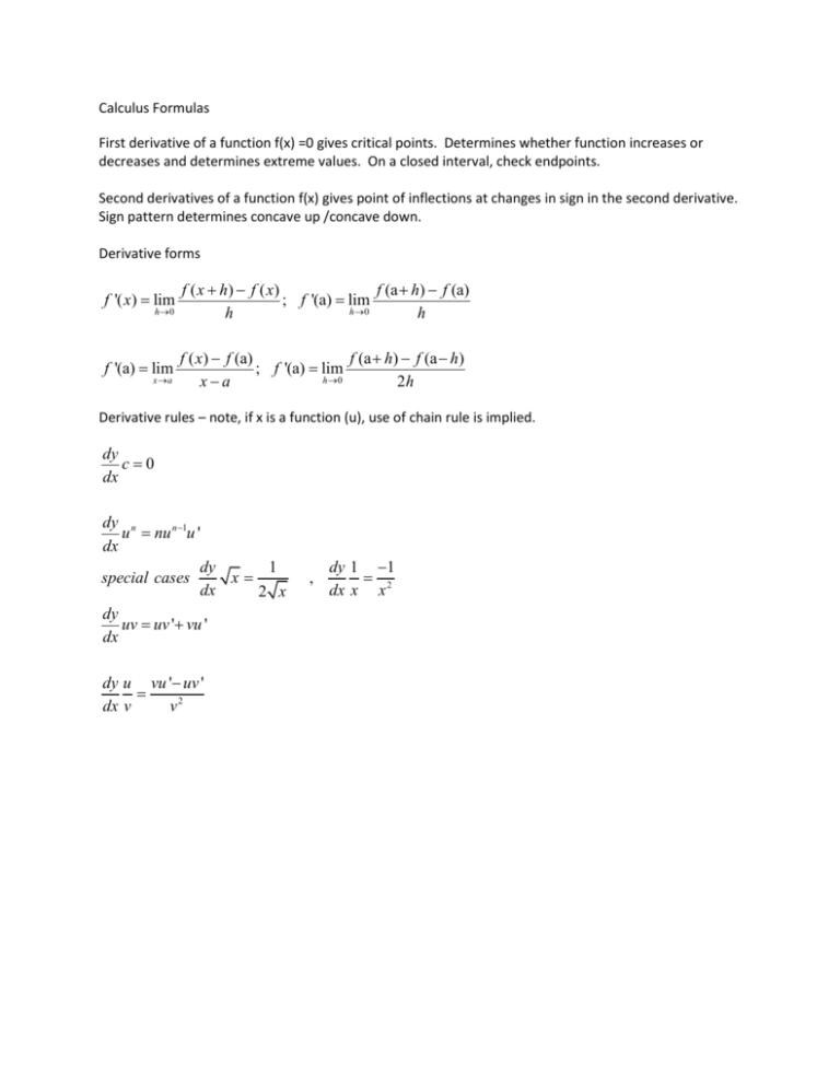
Calculus Formulas First derivative of a function f(x) =0 gives critical points. Determines whether function increases or decreases and determines extreme values. On a closed interval, check endpoints. Second derivatives of a function f(x) gives point of inflections at changes in sign in the second derivative. Sign pattern determines concave up /concave down. Derivative forms f '( x) lim f ( x h) f ( x ) f (a h) f (a) ; f '(a) lim h 0 h h f '(a) lim f ( x) f (a) f (a h) f (a h) ; f '(a) lim h 0 xa 2h h 0 x a Derivative rules – note, if x is a function (u), use of chain rule is implied. dy c0 dx dy n u nu n 1u ' dx dy 1 special cases x dx 2 x dy uv uv ' vu ' dx dy u vu ' uv ' dx v v2 , dy 1 1 dx x x 2 dy sin x cos x dx dy cos x sin x dx dy tan x sec 2 x dx dy sec x sec x tan x dx dy csc x csc x cot x dx dy cot x csc 2 x dx dy 1 tan 1 x dx 1 x2 dy 1 1 sin x dx 1 x2 dy sec 1 x dx x 1 x2 1 inverse cot x, cos x, and csc x are each the opposite of theinverse tan x,sin x, and sec x dy x e ex dx dy 1 ln x dx x dy x a a x ln a dx dy 1 log a x dx x ln a Generalized Chain Rule d ( f ( g (x)) f '(g(x)) g'(x) dx Integral formulas c xC x n 1 C n 1 n x e x ex C 1 x ln x C sin kx cos kx C k cos kx sin kx C k sec 2 kx tan kx C k Average Value of any function on [a,b] b 1 f ( x) dx b a a Extreme Value Theorem On a closed continuous interval [a,b], there must be at least one max and one min value. Intermediate Value Theorem On a closed continuous interval [a,b], every value f(c) must be between f(a) and f(b) for all c on [a,b]. - This theorem applies for derivatives as well Mean Value Theorem On closed continuous [a,b], the slope of the secant line must equal the slope of the tangent line at least once. f '(c) f (b) f (a) if c on (a, b) ba FTC x 1) dy f (t )dt f ( x ) , note if the upper limit of integration is a function of x, you must multiply dx a f(x) by the derivative of the upper limit of integration dy dx g ( x) f (t )dt f (g( x)) g'(x) a b 2) f (x) dx F (b) F(a) if F(x) is any antiderivative of f. a Integral Approximations RRAM, LRAM, MRAM – estimates of areas under curves Underestimate if below curve, upper estimate if above curve Trapezoidal Approximations A= 1 h h(b1 b2 ) or trapezoidal rule ( y0 2 y1 2 y2 ..... 2 yn 1 yn ) 2 2 Integral Techniques U-substitution including changing of limits of integration Separation of variables Position Velocity and Acceleration * do not forget initial conditions Derivative of position is velocity Derivative of velocity is acceleration Integral of acceleration is velocity Integral of velocity is position Absolute value of velocity is speed. Displacement is net distance. Total distance is integral absolute value velocity. Inverses- If f(g(x))=x then you have an inverse. An inverse is when x and y are switched in an order pair. If you are trying to find the derivative of an inverse at a point (a,b), it is tangent line to the inverse at (b,a) is y a 1 ( x b) f '(a) 1 and the equation of the f '( a )
