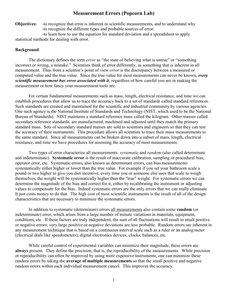
Measurement Errors (Popcorn Lab)
Objectives:
-to recognize that error is inherent in scientific measurements, and to understand why
-to recognize the different types and probable sources of error;
-to learn how to use the equation for standard deviation and a spreadsheet to apply
statistical methods for dealing with error.
Background
The dictionary defines the term error as “the state of believing what is untrue” or “something
incorrect or wrong, a mistake.” Scientists think of error differently, as something that is inherent in all
measurement. Thus from a scientist’s point of view error is the discrepancy between a measured or
computed value and the true value. Since the true value for most measurements can never be known, every
scientific measurement has error associated with it, regardless of how careful you are in making the
measurement or how fancy your measurement tools are.
For certain fundamental measurements such as mass, length, electrical resistance, and time we can
establish procedures that allow us to trace the accuracy back to a set of standards called standard references.
Such standards are created and maintained for the scientific and industrial community by various agencies.
One such agency is the National Institute of Standards and Technology (NIST, which used to be the National
Bureau of Standards). NIST maintains a standard reference mass called the kilogram. Other masses called
secondary reference standards, are manufactured, machined and adjusted until they match the primary
standard mass. Sets of secondary standard masses are sold to scientists and engineers so that they can test
the accuracy of their instruments. This procedure allows all scientists to trace their mass measurements to
the same standard. Since all measurements can be broken down into a subset of mass, length, electrical
resistance, and time we have procedures for assessing the accuracy of most measurements.
Two types of error characterize all measurements: systematic and random (also called determinate
and indeterminate). Systematic error is the result of inaccurate calibration, sampling or procedural bias,
operator error, etc. Systematic errors, also known as determinant errors, can bias measurements
systematically either higher or lower than the true value. For example if you set your bathroom scale a
pound or two higher to give you diet incentive, every time you or someone else uses that scale to weigh
themselves, the weight will be systematically higher than the "true" weight. For systematic errors we can
determine the magnitude of the bias and correct for it, either by recalibrating the instrument or adjusting
values to compensate for the bias. Indeed systematic errors are the only errors that we can really eliminate.
It just costs money to do that. The high cost of most scientific instruments is the result of all of the design
characteristics that are necessary to minimize the systematic errors.
In addition to systematic (determinate) errors all measurements also contain some random (or
indeterminate) error, which arises from a large number of minute variations in materials, equipment,
conditions, etc. If these factors are truly independent, the sum of all fluctuations will result in small positive
or negative errors; very large positive or negative deviations are less probable. Random errors are inherent in
any measurement technique that is based on a continuous interval scale such as a ruler or an analog meter
(electrical dials like speedometers), digital electronics devices, clocks, balances, etc.
While careful control of experimental variables can minimize their magnitude, these errors are
always present. They define the precision, that is, the reproducibility of the measurements. While precision
or reproducibility can often be improved by using more expensive instruments, one can minimize these
random errors by taking the average of multiple measurements so that the small positive and negative
random errors within each individual measurement cancel. This improves the accuracy.
1
The distinction between precision and accuracy is illustrated by the following example: If we liken a
scientist making a measurement to an archer shooting at a target, the "bull's eye" represents the "true" value
of the measurement. Each arrow shot at the target represents a single measurement. Examine Figure 3.1.
The target at the upper left shows that all of the shots are right on target (for simplicity, the arrows are
represented by black dots). Like measurements, the best estimation of the archer's performance is the
average of several shots. Since the average position of all shots is clearly close to the true value (center of
the target) the archer has good accuracy. While all of the shots are in the "bull's eye" there is still some
imprecision because small inherent fluctuations lead to slightly different locations. Since the spread among
the arrows is small and we say that the shots/measurements have high precision. The shots are very
reproducible.
bias
high accuracy
high precision
low accuracy
high precision
bias
high accuracy
low precision
low accuracy
low precision
Figure 3.1 Accuracy and precision.
The target at the upper right simulates another set of measurements. This archer has very good
precision because all of the shots are very close to one another. However, the average position is biased to
the upper right. There is a systematic error. The archer has poor/low accuracy. The error is systematic
because we can measure how far the average is from the true value. (In this example it may be that the sight
on the bow is misaligned.)
The target example shown at the lower left illustrates the results of several shots that have high
accuracy because the average position is right on target. However, the archer has poor precision because the
reproducibility is poor. There is a large spread in the shots. The target at the lower right illustrates the final
possibility. The archer has poor precision and poor accuracy. The average position is off target and the
individual shots have a large spread. The last two cases illustrate why it is important to make many
measurements. It is only after a large number of measurements that all of the random indeterminate errors
cancel out and lead to a good estimate of the true value. When precision is poor, it is very difficult to assess
accuracy. It is usually better to find a way to improve precision rather than to rely on large numbers of
imprecise measures. That is why it often takes so long to establish new scientific discoveries. Repeated
attempts to improve precision and prove reproducibility take time. [Think some more about the scientist-asarcher analogy. What are the differences between the two? That is, where does the analogy break down?
Are these differences important in understanding the process of scientific measurement?]
In this experiment we will examine one of the fundamental characteristics of all measurements.
Namely, the inherent uncertainty in every measurement due to the small random errors in our instruments or
tools that lead to slightly different numbers when we repeat the measurements. We will attempt to
2
characterize two types of popcorn, a generic brand and a gourmet brand. The question is; are the two brands
different in their weights and in the amount of moisture that they contain? Further, we will try to determine
if the amount of moisture contained in the unpopped kernels affects the popping characteristics. Since
popcorn consists of many small units, each differing slightly from others, we will attempt to obtain an
average of several individual kernels of each type. We will compare the average unpopped weight of the two
brands. In order to assess the spread in weights (the reproducibility among kernels), we will calculate the
standard deviation, a statistical estimate of the spread in measurements. Then we will heat the kernels and
determine the weight of water lost through the steam explosion that pops the kernels. Again, we will
calculate the average weight and standard deviations. Then we will use these statistical summaries to make
comparisons and to draw conclusions about the differences between the two brands.
Statistical Background:
This section will contain a rationale as well as a glossary of definitions and formulas for doing
statistical programs. Once you have collected data from a series of measurements, you will enter these data
into a spreadsheet program which will do your calculations for you. Your goal is to analyze the final
statistical results to determine trends and gain understanding of these methods. One way to characterize data
is by identifying what seems to be a typical value. The most common way to define a typical value is by the
mean and the median.

Mean: the average value computed across all cases, sometimes represented with a variable with a line
across the top, e.g. X .

Median: the middle-most value in a set of data.
Which value is more useful? The mean is used more frequently because it can be manipulated
algebraically more easily than the median. However, the mean is more affected by outliers than the median.
An outlier is an extreme value (either due to fact or error) that skews the data in a particular direction. So if
one student gets 100 on a test that the rest of the class does poorly on, that student’s grade will affect the
mean more than the median.
Another characteristic of a distribution of data is its spread—how close the values are to each other.
This is important for the reasons discussed above. In Figure 3.1, the two examples with high precision would
represent experimental data that is not very spread out and would be preferable, in terms of approaching a
“true” value, than if the data were widely distributed. The standard deviation, ()1, is a statistical measure
of the distance a given data point is likely to lie from the average value of the data set. It is mathematically
tedious to calculate but conceptually easy to understand. The standard deviation is a measure of the spread
of data in a distribution, a measure of dispersion. The larger the standard deviation, the further the individual
cases are from the mean (large spread in data). The smaller the standard deviation, the closer the individual
values are to the mean (small spread in data).
Suppose you have two data sets that follow the classic bell curve shown below. The one on the left
has a small standard deviation, meaning all the values are close to the average. The one on the right is more
spread out and has a larger standard deviation.
1
This symbol, , is the Greek lower case sigma.
3
Significant figures and statistics: Frequently, data values are reported in a manner that lists the
mean (average) value first, plus or minus the standard deviation: X ± . The standard deviation should be
expressed to ONE significant figure. The number modified by the significant figure should be expressed to
AGREE IN PLACE with the standard deviation.
Example: Below are two data sets. In Set I, the concentration values have a fairly broad range (from
0.84 M to 1.25M). The standard deviation is also large (0.17). If you calculate the average value with your
calculator you will get 1.022 M (try it and see!). However, the last two digits in this value are not significant
because there is such a large range of values (as reflected by the standard deviation). Thus we can only
confidently report a value of 1.0 M  0.2 M as the concentration of the solution used in this experiment. By
contrast, the values in the second data set are more closely grouped (from 0.98M to 1.05M). Here the
average value is 1.014 M with  = 0.03, so the hundredths decimal in the standard deviation is significant
(but not the thousandths), and we can confidently report 1.01 M  0.03 M as the concentration.
Set I
Run
1
2
3
4
5
Mean

Set II
Conc. (mol/L)
1.15
0.96
0.84
1.25
0.91
Run
1
2
3
4
5
1.022
0.17
Mean

Conc. (mol/L)
1.05
1.03
0.99
1.02
0.98
1.014
0.026
Calculation of Standard Deviation
For the purposes of this lab, you will be given a spreadsheet with pre-programmed formulas. When
you enter your data into the spreadsheet, the means and the standard deviations will be automatically
calculated. In future experiments, however, you will be required to calculate standard deviation using your
calculator – see me for the how-to on using statistics with your graphing calculator. The equation for this is
as follows (without using the graphing calculator) is:
 g 
2

i
n 1
where gi = ( X i  X ) or, the mean subtracted from each individual value
n = total number of values
Using the Set I data from the example above, the equation would be set up as follows:
(1.15  1.022) 2  (0.96  1.022) 2  (0.84  1.022) 2  (1.25  1.022) 2  (0.91  1.022) 2

5 1
You should make this calculation with your calculator to confirm that you get the correct value for
standard deviation (0.017). In a graphing calculator, use STAT, enter the data under L1 in Edit. Then
use STAT, Calc and type in L1. You should get the same results.
Pre-lab Questions – there are videos available on schoology to help with these questions under Ch. 1
and 2 labs.
1. Research the process of popping popcorn on the Internet. Determine the best methods for popping and
what causes the popcorn to pop. Your pre-lab should have a paragraph discussion of popcorn.
4
2. Read over the lab background information and answer the questions below.
a. Using your own words and a few sentences, differentiate between accuracy and precision. Create
your own example to illustrate the difference.
b. Research standard deviation on the internet. What percentage of the sample can be considered to be
within one standard deviation of the mean? Two standard deviations? Three standard
deviations?
c. Based on what you have learned about statistics, why is it important for scientists to make multiple
measurements of data before reporting their average results?
3. The data set below came from a titration. A titration is a common procedure in chemistry for determining
the concentration of a solute in a solution. In this case, an experimentally measured volume of solution A
with a known concentration (0.5000 M) was added to exactly 25.00 mL of solution B of unknown
concentration. The concentration of B is then determined using the MAVA = MBVB
Run
1
2
3
4
Volume of A
added (mL)
44.51
45.01
43.89
44.71
Conc. of B (M)
0.8902
0.9002
0.8778
0.8942
a. i) What value can you confidently report for the average volume of solution A? ii) What value can
you confidently report for the concentration of B?
b. A labeling error occurred and the actual concentration of solution A was 0.4500 M. i) Assuming
that MAVA = MBVB, how would this labeling error affect the calculated values for the concentration
of B? ii) Would this represent a systematic or a random error?
c. If a 5th run were done with a value of 42.05 mL for Volume of A added, would you expect the
standard deviation to increase or decrease? Briefly explain.
4. Set up appropriate data tables based on the procedure below. Model your data tables after the data table
provided in schoology. If you want to type them up on a spreadsheet program, that’s fine. You will need to
have these data tables ready to go on the day of the experiment. Leave plenty of space between data tables in
case you need to take some notes on experimental problems. Leave space to include observations about
relative size of kernels (unpopped and popped) in generic vs. gourmet.
Experimental Procedure:
Note: the actual experimental procedure should take you less time than the scheduled time. You will use the
extra time to start working on the spreadsheet calculations in the computer lab or on your laptop, particularly
since I will be available to help you.
You will be working as a group with the lab partners at the same table as you. One set of partners will collect
data for gourmet popcorn and the other will collect data for generic popcorn.
You will use a numbered well-plate to carry and keep track of your popcorn kernels. Obtain unpopped
kernels from either generic or gourmet popcorn. Place the kernels in the multi-well plate.
Next, you will be determining the mass of each popcorn kernel. It is not necessary to tare the balances, since
you will be determining mass lost from each kernel. These are expensive analytical balances; they read to
0.0001 g, but that last number varies greatly. Don’t spend forever getting it exactly right because even just
leaning on the table can affect the numbers. Determine the mass of each of the kernels individually and
record the mass in your table to the nearest 0.001 gram. Be sure to replace the kernels in the correctly
5
assigned well number. At this point you should have 15 numbered masses for the generic brand kernels and
15 numbered masses for the gourmet brand.
Two suggested ways for popping the kernels:
1) Beaker and flame:
Obtain a dry 100 or 150 mL beaker or one of the metal pots from the counter in the lab. Set up a Bunsen
burner and light it. Adjust the burner to give a low, but stable flame. Wear goggles with this method!
Place one of the kernels into the beaker. Holding the beaker with appropriate tongs, slowly heat the beaker
containing the single kernel until it pops. You should gently shake the beaker back and forth across the flame
to promote even heating and to avoid scorching of the kernel. Immediately after the kernel pops, pour it out
on to the bench top so that it doesn’t burn. Replace this popped kernel in its appropriate numbered well.
Repeat the process until all 15 of the numbered kernels have been popped. Note that this “air popping”
technique may lead to kernels that aren’t as big and fluffy as you are used to seeing in the movie theaters. For
our purposes, “popped” means any kernel which has exploded and released its water contents as steam.
2) Hot Air Popper:
There are four hot air poppers available. Obtain 3 to 5 extra kernels to practice using the hot air popper.
Once you have a technique, you can pop the “official” kernels remembering to weigh before and after
popping. Pop one kernel at a time!
CAUTION! DO NOT EAT THE POPCORN PRODUCED BY EITHER
METHOD. YOU DON'T KNOW WHAT WAS IN THE FLASK/POPPER
PREVIOUSLY, AND THE DESK TOP MAY HAVE HAZARDOUS
CHEMICALS WHICH COULD CONTAMINATE KERNELS.
Continue popping the kernels until you have popped all weighed kernels of each brand. Use the same
balance that you used before to weigh the popped kernels one at a time. Make sure that you record the mass
of the popped kernel next to the pre-popped mass of the same kernel in your lab notebook.
When you are sure that you have accurately determined the mass for each unpopped kernel and the
corresponding mass of the same popped kernel you are finished with the laboratory experimental part of the
experiment.
Before you leave the laboratory, you should exchange data with the group at another lab table so that you
have two complete sets of data.
Calculations:
Before you enter your data into the online spreadsheet in schoology, you should evaluate your data. You
should choose “reasonable” values to enter into the spreadsheet. If a kernel gained mass on popping or if it
remained the same, those are values that are not reasonable and you should not use them in your calculations.
You should also consider eliminating outliers from your data – how you define an outlier is up to you.
In the spreadsheet:

Enter your data for the masses of up to 15 generic unpopped kernels (include the kernel numbers).

Enter your data for the masses of up to 15 generic popped kernels (include the kernel numbers).

Repeat the data entry for the gourmet kernels.

Make sure to save the data for your group using the format defined by the school
(“period#.first.last.assignment name). You can use just last names for this assignment.

Share the data your lab table has with another lab table so that you all have two complete sets of data.
6

Once the spreadsheet has finished the calculations for your data, highlight the data (only yours – not the
table across from you or another table’s data) in the column “mass lost upon popping”, copy and paste it
into the online spreadsheet for the class. There is a link in schoology for class data for period 2 and
period 6. This spreadsheet will calculate a mean and a standard deviation for the entire class and will be
posted for your analysis later.
Report:
Your final lab report should be typed and contain the following, in order:
Title page
A. Purpose – two to three sentences describing what you were attempting to do.
B. Background Information – 1 paragraph (minimum 5 sentences) describing how statistics is used
to analyze sets of data.
C. Spreadsheet of your data and the other group’s data. (Note: on your spreadsheet you should
include mean, median and standard deviation for each column of data calculated by excel).
D. Analysis – Use your calculator or spreadsheet program to calculate the mean, median, and
standard deviation ( X ± ) of ONLY YOUR popcorn sample’s mass lost on popping.
E. Post-lab questions – Answer the questions below.
Answers should be typed; I will show you how to use Insert Equation and Equation Editor to type up your
equations. You could also neatly hand-write the equations and scan it into the document. Make sure I can
read it – pictures of your hand-written work are not a good choice because they are so small.
1. If any of the data were omitted from the calculations because they were unreasonable or outliers, you
should briefly describe why each was omitted.
2. Which type of popcorn shows more variance in kernel size before popping? After popping? In mass loss
upon popping?
3. Compare the standard deviation values calculated for your data with those from the class as a whole (this
data will be posted on the board on the day after lab day and online at schoology).
a) Does the magnitude of the standard deviation “improve” as the size of the data set increases? What
does this tell you?
b) If the magnitude of the standard deviation for the combined data set did not improve, what might
be the reason(s) for this?
4. a) define systematic errors.
b) What was the most significant source of systematic error in the experiment?
c) How did this affect your results?
d) How could you improve the procedure to minimize this error?
5. a) define random errors.
b) What were the most significant sources of random error (at least 2) in this experiment? Vague
statements like “human error” or “incorrect calculations” will not earn credit.
c) How did those random errors (make sure to address both random errors) affect the data you collected?
You should indicate whether the mass (which one – before or after popping) increased or decreased and
why.
6. A student records the following data when determining the density of an unknown solid. She measured the
mass by placing the solid directly on the balance and the volume by water- displacement in a graduated
cylinder.
Trial
Mass (g)
Volume (mL)
Density (g/mL)
1
8.345
12.75
2
12.802
19.55
3
6.395
9.77
a. Calculate the density (in g/mL) for each trial. Show your work for Trial 1 and sig figs for all
trials.
7
b. The balance she used was inaccurately tared. Each measurement of mass was 1.795 g too low. Is
this a systematic or random error? Why?
c. Describe how she could eliminate this error (besides fixing the balance!)
You and your lab partner will write this lab report together. Recommend that one partner writes A, B,
D above and the other does C. You should work on part E above together to come up with the answers. I
suggest either getting together during an off period or going over the answers online in a google doc.
SUBMIT ONE FINAL LAB REPORT ONLINE BY 11:59 PM ON 9/2. You may, of course, take advantage
of tutor time on Monday afternoons and Wednesday mornings to get any assistance from me that you need. I
will arrange for computer access during tutor times if possible.
Popcorn Lab Rubric
Item
Looking for:
Out of
A. Purpose
2 – 3 sentences
2
B. Background
Methods of statistical analysis (5 sentences
minimum each)
3
C. spreadsheet
2
D. Analysis
Calculations
3
E. Postlab
#1 data omitted? Why or why not?
2
#2 more variance before/after and in mass lost
3
#3 comparison of whole class standard dev.
3
#4 two systematic errors, nature, affects and ways
to improve
#5 random errors, nature and affects
4 each = 8
#6 a, b, c
3
Typed, neat, well organized, title page
2
Presentation
Score
4 each = 8
Total______________/39
8