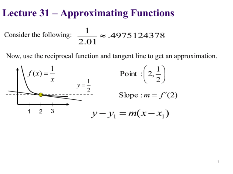
Lecture 31 – Approximating Functions
Consider the following:
1
 .4975124378
2.01
Now, use the reciprocal function and tangent line to get an approximation.
f ( x) 
1
2
1
x
3
y
1
2
 1
Point :  2, 
 2
Slope : m  f ( 2)
y  y1  m( x  x1 )
1
1
 .4975124378
2.01
1
f ( x) 
x
1
y
2
2
1
 L ( 2.01)
2.01
2.01
 1
Point :  2, 
 2
Slope : m  f ( 2)  
L( x)  f (2)  f (2)( x  2)
1
4
2
First derivative gave us more information about the function
(in particular, the direction).
For values of x near a the linear approximation given by the
tangent line should be better than the constant approximation.
Second derivative will give us more information (curvature).
For values of x near a the quadratic approximation should
be better than the linear approximation.
3
What quadratic is used as the approximation?
p2 ( x)  c0  c1 ( x  a)  c2 ( x  a)
2
Key idea: Need to have quadratic match up with the
function and its first and second derivatives at x = a.
4
1
 .4975124378
Use p2(x) to get a better approximation.
2.01
f (a)
2
1
1

p
(
x
)

f
(
a
)

f
(
a
)(
x

a
)

(
x

a
)
f ( x) 
f ( 2) 
2
2
x
2
f ' ( x)  
1
x2
f ' ( 2)  
f '' ( x ) 
2
x3
f '' (2) 
f ( x) 
2
1
x
2.01
1
4
1
4
1
 p2 (2.01)
2.01
5
f ( x)  e
Graphical Example at x = 0
f ( x)  e (2 x)
 x2
 2 xe
 x2
f ( x)  (2 x)(e
e
 x2
 x2
 x2
(2 x))  (e
 x2
)(2)
(4 x  2)
2
p0 ( x) 
p1 ( x) 
p2 ( x) 
6
1
2
3
What higher degree polynomial is appropriate?
Key idea: Need to have nth degree polynomial match up
with the function and all of its derivatives at x = a.
pn ( x)  c0  c1 ( x  a)  c2 ( x  a)    cn ( x  a)
2
n
pn' ( x) 
pn'' ( x) 
pn
( n)
( x) 
7
The coefficients, ck, for the nth degree Taylor polynomial
approximating the function f(x) at x = a have the form:
n
p n ( x )   ck ( x  a ) 
k
k 0
8
Lecture 32 – Taylor Polynomials
Def: The Taylor polynomial of order n for function f at x = a:
k 
n
pn ( x )  
f
k 0
(a)
k
( x  a)
k!
The remainder term for using this polynomial:
Rn ( x)  f ( x)  pn ( x)
for some c between x and a.
where M provides a bound on
how big the n+1st derivative
could possibly be.
9
Estimate the maximum error in approximating the reciprocal
function at x = 2 with an 8th order Taylor polynomial on the
interval [2, 3].
1
f ( x) 
x
1
f ' ( x)   2
x
(8)
f (2)
f
(2)
2

p8 ( x)  f (2)  f (2)( x  2) 
( x  2)   
( x  2)8
2!
8!
R8 ( x) 
f
(9)
(c )
9
( x  2)
9!
2
f '' ( x )  3
x
6
f ''' ( x)   4
x
f
( 4)
24
( x)  5
x
10
Rn ( x)  M
R8 ( x) 
f
xa
(n  1)!
| x2|
(c )
9
( x  2)  M
9!
9!
(9)
n 1
9
11
What is the actual maximum error in approximating the
reciprocal function at x = 2 with an 8th order Taylor
polynomial on the interval [2, 3]?
1
f ( x) 
x
(8)
f (2)
f
(2)
p8 ( x)  f (2)  f (2)( x  2) 
( x  2) 2   
( x  2)8
2!
8!
R8 (3)
1
  p8 (3) 
3
12
What nth degree polynomial would you need in order to
keep the error below .0001?
1
f ( x) 
x
(n)
f (2)
f
(2)
2

pn ( x)  f (2)  f (2)( x  2) 
( x  2)   
( x  2) n
2!
n!
( n 1)
f
(c)
Rn ( x) 
( x  2) n1
(n  1) !
f
(n)
n!
( x)  (1) n 1
x
n
f
( n 1)
( x)  (1)
n 1
n  1!
x n2
13
( n 1)
f
(c )
n 1
Rn ( x) 
( x  2)
(n  1) !
To keep error below .0001, need to keep Rn below .0001.
14
Lecture 33 – Taylor Series
The Taylor series centered at x = a:
n 


f
n 0
is a power series with
(a)
n
( x  a)
n!
cn 
f
(n)
(a)
n!
The Taylor series centered at x = 0 is called a Maclaurin series:


n 0
f
n 
(0) n
x
n!
15
Example 1 Find the Maclaurin series for f (x) = sin x.
f ( x)  sin x f ' ( x)  cos x f '' ( x)   sin x f ''' ( x)   cos x f ( 4) ( x)  sin x

sin x  
n 0
f
n 
(0) n
x
n!
f (0) 2
f ( k ) (0) k
 f (0)  f (0) x 
x 
x 
2!
k!
16
Example 2 Find the Maclaurin series for f (x) = ex.
f ' ( x)  e x
f ( x)  e x

e 
x
n 0
f
f '' ( x)  e x
f ( n ) ( x)  e x
n 
(0) n
x
n!
f (0) 2
f ( k ) (0) k
 f (0)  f (0) x 
x 
x 
2!
k!
17
For what values of x will the last two series converge?
x 2 k 1
sin x  
k 0 (2k  1) !


x 2 n 3
2n  1!
lim

n  ( 2n  3)!
x 2 n 1
Ratio Test:
Series converges for

k
x
e 
k 0 k !
x
Series converges for
x n 1 n !
lim
 n 
n  ( n  1)! x
18
y1  x
Consider the graphs:
3
5
7
x
x
x
sin x  x     
3! 5! 7 !
1
x3
y3  x 
63
x
x5
y5  x  
6 120
3
5
7
x
x
x
y7  x  

6 120 5040
19
Example 3 Find the Maclaurin series for f (x) = ln(1 + x).
f ( x)  ln( 1  x) f ' ( x) 

ln( 1  x)  
n 0
f
1
1 x
f '' ( x)  
1
1  x 2
f ''' ( x) 
2
6
( 4)
f
(
x
)


(1  x) 4
1  x 3
n 
(0) n
x
n!
f (0) 2
f ( k ) (0) k
 f (0)  f (0) x 
x 
x 
2!
k!
20
For what values of x will the series converge?
2
3
4

k
x
x
x
k 1 x
ln( 1  x)  x         1
2 3 4
k
k 1
x n 1 n
lim
 n 
n  n  1 x
21
Example 4

k
x
x
x
x
x
e  1 x 


  
2 ! 3! 4 !
k 0 k !
2
3
4
Creating new series for:
f ( x)  e
 x2
22
Lecture 34 – More Taylor Series
Create and use other Taylor series like was done with power series.
sin x
2 k 1

(1) x
x3 x5 x7
 x 

 
3! 5! 7 !
k 0 (2k  1) !

k
cos x
cos x
23
Example 1
cos x
x x 2 x3
 1 
 
2! 4! 6!
2 cos x  2  x
lim
2
x 
x
2 cos x
2 cos x  2  x
2 cos x  2  x
x2
24
Example 2
x 2 x3 x 4
ln( 1  x)  x     ...
2 3 4
 3
lim x ln 1  
x 
 x
25
Example 3
e
x
2
3
4
x
x
x
 1 x 


 
2 ! 3! 4 !

k
x

k 0 k !
ex
 x dx
26
Example 4
1
sin x

(1) k x 2 k 1
x3 x5 x7
 x 

  
3! 5! 7 !
k 0 (2k  1) !
sin(
x
)
dx
 .3102683
0
2
27
Example 5

.2
0
x 2 x3 x 4
ln( 1  x)  x     ...
2 3 4
ln( 1  t )
dt  .19080014
t
28