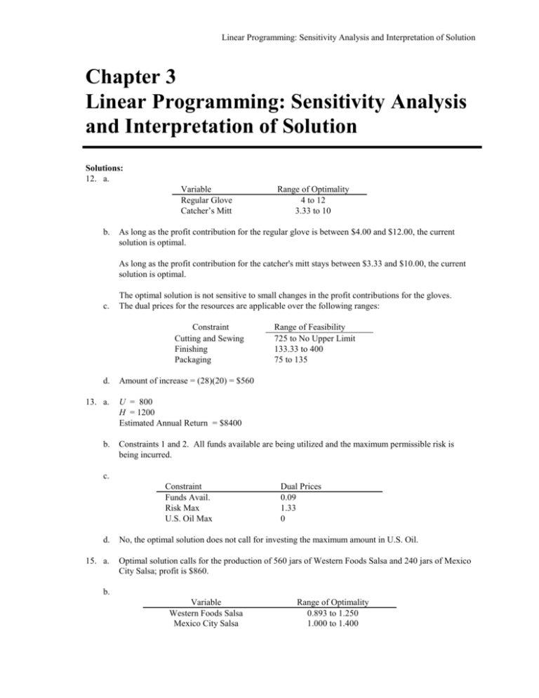
Linear Programming: Sensitivity Analysis and Interpretation of Solution
Chapter 3
Linear Programming: Sensitivity Analysis
and Interpretation of Solution
Solutions:
12. a.
Variable
Regular Glove
Catcher’s Mitt
b.
Range of Optimality
4 to 12
3.33 to 10
As long as the profit contribution for the regular glove is between $4.00 and $12.00, the current
solution is optimal.
As long as the profit contribution for the catcher's mitt stays between $3.33 and $10.00, the current
solution is optimal.
c.
The optimal solution is not sensitive to small changes in the profit contributions for the gloves.
The dual prices for the resources are applicable over the following ranges:
Constraint
Cutting and Sewing
Finishing
Packaging
d.
13. a.
b.
Range of Feasibility
725 to No Upper Limit
133.33 to 400
75 to 135
Amount of increase = (28)(20) = $560
U = 800
H = 1200
Estimated Annual Return = $8400
Constraints 1 and 2. All funds available are being utilized and the maximum permissible risk is
being incurred.
c.
Constraint
Funds Avail.
Risk Max
U.S. Oil Max
d.
15. a.
Dual Prices
0.09
1.33
0
No, the optimal solution does not call for investing the maximum amount in U.S. Oil.
Optimal solution calls for the production of 560 jars of Western Foods Salsa and 240 jars of Mexico
City Salsa; profit is $860.
b.
Variable
Western Foods Salsa
Mexico City Salsa
Range of Optimality
0.893 to 1.250
1.000 to 1.400
Chapter 3
c.
Constraint
1
Dual Price
0.125
2
0.000
3
0.187
Interpretation
One more ounce of whole tomatoes will increase profits by
$0.125
Additional ounces of tomato sauce will not improve profits;
slack of 160 ounces.
One more ounce of tomato paste will increase profits by $0.187
d.
Constraint
1
2
3
17. a.
Range of Feasibility
4320 to 5600
1920 to No Upper Limit
1280 to 1640
No change in optimal solution; there is no upper limit for the range of optimality for the objective
coefficient for S.
b.
No change in the optimal solution; the objective coefficient for M can increase to 6.4.
c.
There is no upper limit on the allowable increase for CS ; thus the percentage increase is 0%.
For C M , we obtain 0.3/3.4 = 0.088 The accumulated percentage change is 8.8%. Thus, the 100%
rule is satisfied and the optimal solution will not change.
18. a.
E = 80, S = 120, D = 0
Profit = $16,440
b.
Fan motors and cooling coils
c.
Labor hours; 320 hours available.
d.
Objective function coefficient range of optimality
No lower limit to 159.
Since $150 is in this range, the optimal solution would not change.
19. a.
Range of optimality
E
S
D
47.5 to 75
87 to 126
No lower limit to 159.
b.
Model
E
S
D
Profit
$63
$95
$135
Change
Increase $6
Decrease $2
Increase $4
Allowable
Increase/Decrease
$75 - $63 = $12
$95 - $87 = $8
$159 - $135 = $24
%
6/12 = 0.50
2/8 = 0.25
4/24 = 0.17
0.92
Linear Programming: Sensitivity Analysis and Interpretation of Solution
Since changes are 92% of allowable changes, the optimal solution of E = 80, S = 120, D = 0 will not
change.
However, the change in total profit will be:
E 80 unit @ + $6 =
S 120 unit @ - $2 =
$480
-240
$240
 Profit = $16,440 + 240 = 16,680.
c.
Range of feasibility
Constraint 1
Constraint 2
Constraint 3
d.
160 to 180
200 to 400
2080 to No Upper Limit
Yes, fan motors = 200 + 100 = 300 is outside the range of feasibility.
The dual price will change.
20. a.
b.
Manufacture 100 cases of model A
Manufacture 60 cases of model B
Purchase 90 cases of model B
Total Cost = $2170
Demand for model A
Demand for model B
Assembly time
c.
Constraint
1
2
3
4
Dual Price
-12.25
-9.0
0
.375
If demand for model A increases by 1 unit, total cost will increase by $12.25
If demand for model B increases by 1 unit, total cost will increase by $9.00
If an additional minute of assembly time is available, total cost will decrease by $.375
d.
The assembly time constraint. Each additional minute of assembly time will decrease costs by $.375.
Note that this will be true up to a value of 1133.33 hours.
Some students may say that the demand constraint for model A should be selected because
decreasing the demand by one unit will decrease cost by $12.25. But, carrying this argument to the
extreme would argue for a demand of 0.
21. a.
Decision Variable
AM
BM
AP
BP
Ranges of Optimality
No lower limit to 11.75
3.667 to 9
12.25 to No Upper Limit
6 to 11.333
Chapter 3
b.
Provided a single change of an objective function coefficient is within its above range, the optimal
solution AM = 100, BM = 60, AP = 0, and BP = 90 will not change.
This change is within the range of optimality. The optimal solution remains AM = 100, BM = 60, AP
= 0, and BP = 90. The $11.20 - $10.00 = $1.20 per unit cost increase will increase the total cost to
$2170 = $1.20(100) = $2290.
c.
Variable
AM
BM
Cost
10
6
Change
Increase 1.20
Decrease 1
Allowable
Increase/Decrease
11.75 - 10 = 1.75
6.0 - 3.667 = 2.333
Percentage
Change
(1.20/1.75)100 = 68.57
(1/2.333)100 = 42.86
111.43
111.43% exceeds 100%; therefore, we must resolve the problem.
Resolving the problem provides the new optimal solution: AM = 0, BM = 135, AP = 100, and BP =
15; the total cost is $22,100.
22. a.
All Pro:
1000
College:
200
High School:
0
b.
The sewing constraint and the minimum production requirement for the All Pro model.
c.
Constraint 1: There are 4000 minutes of unused cutting and dyeing time.
Constraint 2: All the sewing time is being utilized at the optimal solution.
Constraint 3: There are 5200 minutes of unused inspection and packaging time.
Constraint 4: Only the minimum number of All-Pro models is being produced.
d.
Variable
A
C
H
Range of Optimality
No Lower Limit to 5
5 to No Upper Limit
No Lower Limit to 4
No amount of decrease in the profit contribution for the All Pro and High School models will cause
the optimal solution to change. A small decrease in the profit contribution for the College model will
cause the optimal solution to change. A small increase in the profit contribution for the High School
model will cause a change in the optimal solution.
24. a.
b.
Let
H = amount allocated to home loans
P = amount allocated to personal loans
A = amount allocated to automobile loans
Max
0.07H + 0.12P + 0.09A
s.t.
H +
P +
A = 1,000,000
0.6H 0.4P 0.4A  0
P 0.6A  0
H = $400,000 P = $225,000 A = $375,000
Total annual return = $88,750
Amount of New Funds
Minimum Home Loans
Personal Loan Requirement
Linear Programming: Sensitivity Analysis and Interpretation of Solution
Annual percentage return = 8.875%
c.
The range of optimality for H is No Lower Limit to 0.101. Since 0.09 is within the range of
optimality, the solution obtained in part (b) will not change.
d.
The dual price for constraint 1 is 0.089. The range of feasibility for constraint 1 is 0 to No Upper
Limit. Therefore, increasing the amount of new funds available by $10,000 will increase the total
annual return by 0.089 (10,000) = $890.
e.
The second constraint now becomes
-0.61H - 0.39P - 0.39A  0
The new optimal solution is
H = $390,000 P = $228,750 A = $381,250
Total annual return = $89,062.50, an increase of $312.50
Annual percentage return = 8.906%, an increase of approximately 0.031%.
29. a.
Let
O1
O2
O3
C1
C2
C3
=
=
=
=
=
=
percentage of Oak cabinets assigned to cabinetmaker 1
percentage of Oak cabinets assigned to cabinetmaker 2
percentage of Oak cabinets assigned to cabinetmaker 3
percentage of Cherry cabinets assigned to cabinetmaker 1
percentage of Cherry cabinets assigned to cabinetmaker 2
percentage of Cherry cabinets assigned to cabinetmaker 3
Min 1800 O1 + 1764 O2 + 1650 O3 + 2160 C1 + 2016 C2 + 1925 C3
s.t.
50 O1
+
60 C1
42O2
+ 48 C2
30 O3
+ 35 C3
O1 +
O2 +
O3
C1 +
C2 +
C3
O1, O2, O3, C1, C2, C3  0



=
=
40
30
35
1
1
Hours avail. 1
Hours avail. 2
Hours avail. 3
Oak
Cherry
Note: objective function coefficients are obtained by multiplying the hours required to complete all
the oak or cherry cabinets times the corresponding cost per hour. For example, 1800 for O1 is the
product of 50 and 36, 1764 for O2 is the product of 42 and 42 and so on.
b.
Oak
Cherry
c.
d.
e.
Cabinetmaker 1
O1 = 0.271
C1 = 0.000
Cabinetmaker 2
O2 = 0.000
C2 = 0.625
Cabinetmaker 3
O3 = 0.729
C3 = 0.375
Total Cost = $3672.50
No, since cabinetmaker 1 has a slack of 26.458 hours. Alternatively, since the dual price for
constraint 1 is 0, increasing the right hand side of constraint 1 will not change the value of the
optimal solution.
The dual price for constraint 2 is 1.750. The upper limit on the range of feasibility is 41.143.
Therefore, each additional hour of time for cabinetmaker 2 will reduce total cost by $1.75 per hour,
up to a maximum of 41.143 hours.
The new objective function coefficients for O2 and C2 are 42(38) = 1596 and 48(38) = 1824,
respectively. The optimal solution does not change but the total cost decreases to $3552.50.