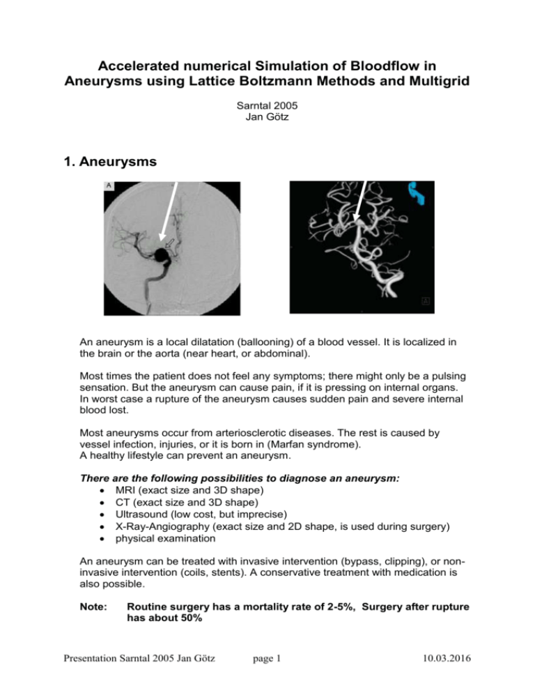
Accelerated numerical Simulation of Bloodflow in
Aneurysms using Lattice Boltzmann Methods and Multigrid
Sarntal 2005
Jan Götz
1. Aneurysms
An aneurysm is a local dilatation (ballooning) of a blood vessel. It is localized in
the brain or the aorta (near heart, or abdominal).
Most times the patient does not feel any symptoms; there might only be a pulsing
sensation. But the aneurysm can cause pain, if it is pressing on internal organs.
In worst case a rupture of the aneurysm causes sudden pain and severe internal
blood lost.
Most aneurysms occur from arteriosclerotic diseases. The rest is caused by
vessel infection, injuries, or it is born in (Marfan syndrome).
A healthy lifestyle can prevent an aneurysm.
There are the following possibilities to diagnose an aneurysm:
 MRI (exact size and 3D shape)
 CT (exact size and 3D shape)
 Ultrasound (low cost, but imprecise)
 X-Ray-Angiography (exact size and 2D shape, is used during surgery)
 physical examination
An aneurysm can be treated with invasive intervention (bypass, clipping), or noninvasive intervention (coils, stents). A conservative treatment with medication is
also possible.
Note:
Routine surgery has a mortality rate of 2-5%, Surgery after rupture
has about 50%
Presentation Sarntal 2005 Jan Götz
page 1
10.03.2016
pictures of a stent.model (left) and a real
stent (right)
2. Numerical Basics
2.1 What is the Lattice Boltzmann method?
1. can be imagined as a type of cellular automaton
2. divide simulation region into a cartesian grid of
square/cubic cells
3. each cell only interacts with its direct
neighbourhood
4. first order explicit discretization (in space and time)
of the Boltzmann equation in a discrete phase
space, which describes all molecules with their
corresponding velocities
Example: D3Q19 is a model for 3 dimensions with 19 velocity-directions
2.2 Equations
f

1
1. Collide step
f a* ( xi , yi )  f a ( xi , yi ) 
2. Stream step
f an 1 ( xi  hea1 , yi  hea2 )  f a* ( xi , yi )
Presentation Sarntal 2005 Jan Götz
page 2
n
a
( xi , yi )  f aeq ( xi , yi )
n

10.03.2016
How to calculate the equilibrium distribution?
3
9

2
f aeq  wa    3ea  u  u 2  ea  u  
2
2


eq
   fa   fa
u   ea f a   ea f aeq
a
a
a
wi 1 / 3 for i  1
wi 1 / 18 for i  2,7
wi 1 / 36 for i  8,19
a
2.3 Multigrid
We use the full approximation storage (FAS) for the nonlinear problem.
FAS equations
LH uH  LH IˆhH uh   I hH Rh (uh )
LH uH  LH IˆhH uh  I hH Rh (uh )

uhn1  uhn  I Hh uH  IˆhH uhn

2.4 Simplifications
a)
Blood is a suspension of formed blood cells and some liquid particles in
an aqueous solution
At high shear rate (γ<100 sec-1) blood can be treated as Newtonian
We focus on large vessels
→ here are high shear rates
b)
Fluid-structure interaction
We neglect the effect of elastic walls.
This is reasonable, because in large arteries the effect is quite minor.
Additionally, we assume blood as homogenous and incompressible.
3. Simulation
3.1 Goal of the Simulation
Recall:
Routine surgery has a mortality rate of 2-5%, but a surgery after rupture has
about 50%!!!
And:
Presentation Sarntal 2005 Jan Götz
page 3
10.03.2016
The number one cause of death in a developed nation is a heart- or vascular
disease
→ simulations of hemodynamics are very important
We want to calculate a time-independent incompressible velocity-field and
use this as an initial guess for a periodically forced time-dependent velocityfield
3.2 Why Lattice Boltzmann ?
1. LBM results in an accurate reproduction of the Navier-Stokes-equations, so
why NOT ?
2. very complex geometries are readily handled
3. LBM is simple to implement and modify
4. changing the geometry during simulation is possible
5. calculate pressure and other stresses locally in time and space
6. very good parallelization, vectorization and cach-optimazation
3,3 The algorithm
f

1
1. Collide step
f a* ( xi , yi )  f a ( xi , yi ) 
2. Stream step
f a** ( xi  hea1 , yi  hea2 )  f a* ( xi , yi )
3. Relaxation
f an 1   f a**  DH  1    f an

n
a
( xi , yi )  f aeq ( xi , yi )
n

DH is called the defect correction
How to get the defect correction ???
1.
 1
Rh  f   f a* ( xi , yi )  1   f a ( xi  hea1 , yi  hea2 )
 
1
 f aeq ( xi  hea1 , yi  hea2 )

2.


DH  RH IˆhH f h  2I hH Rh  f h 
Presentation Sarntal 2005 Jan Götz
page 4
10.03.2016
