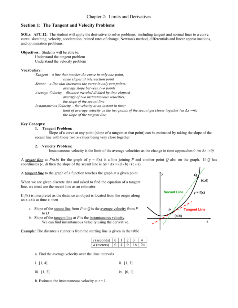
Chapter 2: Limits and Derivatives
Section 1: The Tangent and Velocity Problems
SOLs: APC.12: The student will apply the derivative to solve problems, including tangent and normal lines to a curve,
curve sketching, velocity, acceleration, related rates of change, Newton's method, differentials and linear approximations,
and optimization problems.
Objectives: Students will be able to:
Understand the tangent problem
Understand the velocity problem
Vocabulary:
Tangent – a line that touches the curve in only one point;
same slopes at intersection point
Secant – a line that intersects the curve in only two points;
average slope between two points
Average Velocity – distance traveled divided by time elapsed
average of two instantaneous velocities;
the slope of the secant line
Instantaneous Velocity – the velocity at an instant in time;
limit of average velocity as the two points of the secant get closer together (as ∆x →0)
the slope of the tangent line
Key Concepts:
1. Tangent Problem:
Slope of a curve at any point (slope of a tangent at that point) can be estimated by taking the slope of the
secant line with those two x-values being very close together
2.
Velocity Problem:
Instantaneous velocity is the limit of the average velocities as the change in time approaches 0 (as ∆t →0)
A secant line at P(a,b) for the graph of y = f(x) is a line joining P and another point Q also on the graph. If Q has
coordinates (c, d) then the slope of the secant line is ∆y / ∆x = (d - b) / (c - a).
A tangent line to the graph of a function touches the graph at a given point.
y
Q
(c,d)
When we are given discrete data and asked to find the equation of a tangent
line, we must use the secant line as an estimator.
Secant Line
If f(x) is interpreted as the distance an object is located from the origin along
an x-axis at time x, then
a. Slope of the secant line from P to Q is the average velocity from P
to Q
b. Slope of the tangent line at P is the instantaneous velocity.
We can find instantaneous velocity using the derivative.
0
0
1
4
2
9
3
16
a. Find the average velocity over the time intervals
i. [1, 4]
ii. [1, 3]
iii. [1, 2]
iv. [0, 1]
b. Estimate the instantaneous velocity at t = 1.
Tangent Line
P
(a,b)
x
Example: The distance a runner is from the starting line is given in the table
t (seconds)
d (meters)
y = f(x)
4
24
Chapter 2: Limits and Derivatives
Tangent versus Secant Lines
y
1
∆y 17-2 15
m 1 = ---- = ------ = ---∆x 12-3
9
2
Se
ca
nt
(x² + 9)
y = ---------9
Se
ca
nt
∆y 10-2 8
m 2 = ---- = ------ = --∆x
9-3 6
∆y 5-1
4
m t = ---- = ------ = --∆x 6-0
6
c
Se
an
t3
∆y
5-2
3
m 3 = ---- = ------ = --∆x
6-3
3
x
Tangent versus Secant Lines
y
∆y 17-1 16
m 1 = ---- = ------ = ---∆x 12-0 12
Se
ca
nt
1
(x² + 9)
y = ---------9
∆y 5-1
4
m t = ---- = ------ = --∆x 6-0
6
Se
ca
nt
2
∆y 10-1 1
m 2 = ---- = ------ = --∆x
9-0 1
c
Se
an
t3
∆y
5-1
4
m 3 = ---- = ------ = --∆x
6-0
6
x
Concept Summary:
The slope of the secant approaches the slope of the tangent at a point on the curve as ∆x →0
Homework – Problems: pg 91-92: 1, 5, 8
Read: Section 2.2
Skills for Next Section: Limits
Chapter 2: Limits and Derivatives
Section 2: The Limit of a Function
SOLs: APC.2: The student will define and apply the properties of limits of functions. This will include limits of a constant,
sum, product, quotient, one-sided limits, limits at infinity, infinite limits, and nonexistent limits.
Objectives: Students will be able to:
Determine and Understand one-sided limits
Determine and Understand two-sided limits
Vocabulary:
Limit (two sided) – as x approaches a value a, f(x) approaches a value L
Left-hand (side) Limit – as x approaches a value a from the negative side, f(x) approaches a value L
Right-hand (side) Limit – as x approaches a value a from the positive side, f(x) approaches a value L
DNE – does not exist (either a limit increase/decreases without bound or the two one-sided limits are not equal)
Infinity – increases (+∞) without bound or decreases (-∞) without bound [NOT a number!!]
Vertical Asymptote – at x = a because a limit as x approaches a either increases or decreases without bound
Key Concepts:
Limits
When we look at the limit below, we examine the f(x) values as x gets very close to a:
lim f(x) = L
read: the limit of f(x), as x approaches a, equals L
xa
One-Sided Limits:
Left-hand limit (as x approaches a from the left side – smaller)
lim f(x) = L
xa-
RIght-hand limit (as x approaches a from the right side – larger)
lim f(x) = L
xa+
The two-sided limit (first one shown) = L if and only if both one-sided limits = L
lim f(x) = L
if and only if
lim f(x) = L and lim f(x) = L
xa-
xa
xa+
Vertical Asymptotes:
The line x = a is called a verticle asymptote of y = f(x) if at least one of the following is
true: lim f(x) = ∞
lim f(x) = ∞
lim f(x) = ∞
xa-
xa
lim f(x) = -∞
lim f(x) = -∞
xa
Limits
-
xa
Usually a reasonable
guess would be:
xa+
lim f(x) = -∞
xa+
y
One Sided Limits
Limit from right:
lim f(x) = f(a)
lim f(x) = 5
xa
x10+
(this will be true for
continuous functions)
ex:
Limit from left:
lim f(x) = 3
lim f(x) = 2
x10-
x2
but,
Since the two onesided limits are not
equal, then
lim f(x) = 7
x5
(not f(5) = 1)
and lim f(x) = DNE
x
x16
(DNE = does not exist)
2
5
10
lim f(x) = DNE
x10
15
When we look at the limit below, we examine
the f(x) values as x gets very close to a:
lim f(x)
xa
Remember: around a point where a function does not exist, trying to guess the limit may have some pitfalls as examples 2
through 6 go through in the book. A calculator is not a replacement for a thinking mind!
Chapter 2: Limits and Derivatives
lim f ( x)  L
means that as x gets closer and closer to the number a (but not
x a
equal to a), the corresponding f(x) values get closer and closer to the number L.
Example 1: Answer each using the graph to the right (from Study Guide that
accompanies Single Variable Calculus by Stewart)
a.
lim f  x  
b.
lim f  x  
d.
x 5
c.
lim f  x  
x 2
x 0
lim f  x  
x 4
sin x
x 0
x
lim
2. Use tables to estimate
3. Use algebra to find:
x3  1

x 1 x  1
b. lim
a. lim
x 1
x 1
x 1

1 
 x


c. lim 
x 1 x  1
x  1 
Look at page 94-95, ex 4 & 5 for two tricky limits.
lim f  x   L , the left-hand limit of f at a means that f(x) gets closer and closer to L as x approaches a and x < a. It is
called “left-hand” because it only concerns values of x less than a (to the left of a on the x-axis)
xa 
lim f x  L , the right-hand limit is a similar concept but involves only values of x greater than a.
xa 
lim f  x  both exist and are the same number L, then
If lim f  x  and
xa 
xa
 and equals L.
lim f  xexists
x a
If either one sided limit does not exist or, or they exist but are different numbers, then
If lim f  x   L
xa
Examples:
a.
d.
g.
1. Use the graph to answer each of the following:
b.
lim f  x  
e.
lim f  x  
h.
x 2
x 0

x a
, then both one sided limits exist and are equal to L. (see page 98 for diagrams)
lim f  x  
x 2
lim f  x does not exist.
lim f  x  
c.
lim f  x  
f.
lim f  x  
i.
x 2

x 2

x 0

lim f  x  
x 2

lim f  x  
x 2

lim f  x  
x 0
Chapter 2: Limits and Derivatives
2.
lim
x 3
3 x

x 3
3x  1
x2
x2  3

x2
x2

3. Find, lim f  x   where f  x    8
x 2
4. Always, sometimes, or never true:
 not exist.
lim f  xdoes
lim f  x  does not exist, then
a. If
x2
x 2 
x 2 
x2
lim f  x  does not exist, then
b. If
lim f  x does not exist.
Sometimes lim f x 
does not exist because as x is assigned values that approach a the corresponding f(x) values grow
xa
larger without
bound. In this case we say:
lim f x  
xa
Remember:

lim f x    still means the limit does not exist, but it fails to exist in this special way – we get a direction!
xa
The graph goes up without bound.
lim f x    means f(x) becomes smaller without bound as x approaches a, but the graph goes off in the
xa
opposite direction.
Example: Evaluate the limits given the graph of f(x) :
a.
lim f  x  
f.
lim f  x  
g.
lim f  x  
h.
lim f  x  
i.
x 2
b.
x 2
c.
x 3
e.
lim f  x  
x 0

x 2
d.
lim f  x  
x 3


lim f  x  
x 0

lim f  x  
x 0

lim f  x  
x 3

True/False:

If lim f x  
xa
and
lim g x    , then
xa
lim  f x  . g x   0
xa
Homework – Problems: pg 102-104: [Day 1] 5, 6, 7, 9; [Day 2] 12, 19, 21, 23, 24, 27
Read: Section 2.3
Skills for Next Section: Laws of Limits
Chapter 2: Limits and Derivatives
Section 3: Calculating Limits Using the Limit Laws
SOLs: APC.2: The student will define and apply the properties of limits of functions. This will include limits of a constant,
sum, product, quotient, one-sided limits, limits at infinity, infinite limits, and nonexistent limits.
Objectives: Students will be able to:
Find Limits using the laws of Limits
Understand and use the Squeeze Theorem
Vocabulary:
Greatest Integer Function – [[ x ]], the largest integer that is less than or equal to x
Continuous – (studied in detail in 2.5) no interrupt or abrupt change in the function
Key Concept:
Laws of Limits Summary
lim f(x)
Suppose c is a constant and the
lim g(x)
and
xa
1. lim [f(x) + g(x)] =
lim f(x) + lim g(x)
xa
xa
2. lim [f(x) - g(x)] =
lim g(x)
xa
Difference Law
xa
= c lim f(x)
xa
Constant Multiple Law
xa
4. lim [f(x) • g(x)]
lim f(x) • lim g(x)
=
xa
xa
5. lim [f(x) / g(x)]
=
lim g(x) , if lim g(x) ≠ 0
xa
6. lim [f(x)]ⁿ
=
xa
[lim f(x)]ⁿ
xa
Product Law
xa
lim f(x) /
xa
Quotient Law
xa
from Product
(n is a positive integer)
xa
7. lim c = c
lim x
8.
Special Limits
=a
xa
xa
9. lim xⁿ = aⁿ
ⁿ = √a
ⁿ
lim √x
10.
from 6 and 8
xa
xa
ⁿ
11. lim √f(x)
Sum Law
xa
lim f(x) -
xa
3. lim [cf(x)]
exist. Then ---
xa
=
ⁿ√lim f(x)
xa
Generalization
xa
Squeeze Theorem
Theorem: If f(x) ≤ g(x) when x is near a (except possibly at a) and the limits of f and g
exist as x approaches a, then
lim f(x)
≤
lim g(x)
xa
xa
SQUEEZE THEOREM:
(Conditions:) 1) If f(x) ≤ g(x) ≤ h(x) when x is near a (except possibly at a) and
2) lim f(x)
=
lim h(x)
xa
then
=
L
y
xa
y = x²
lim g(x) = L
xa
y = x² sin (1/x)
Figure 8 from pg 111
x
y = -x²
Chapter 2: Limits and Derivatives
Examples: Find each of the following
1.

lim 4 x 2  10x  3
x 6
3.

 x2  6x  5 

 x 1 
2. lim 
x 1
 2
4. lim f  x  where f x    x
x 3
x3
6 x  4 x  3
4 x  44
lim 3
x5 6 x  29
 f  g x 
5. lim
x 2
6.
1

 x

lim  x
x 1  1


1


 x

7.

lim 
x 0

given
2 x  2 


x

If a function g(x) is “trapped” or “sandwiched” or “squeezed” between two functions f(x) and h(x) with a known limit L as x
approaches c, then the limit of g(x) will also be L. This is called the squeeze theorem – look on page 110 for the formal
definition and page 111 for the picture.
This theorem allows us to find limits of strange functions and to prove some limits analytically.
Prove:
lim
 0
sin 

1
Homework – Problems: pg 111-113: [Day 1] 1, 3, 6, 10, 11, 13, 20 [Day 2] 33, 40, 41, 52
Read: Section 2.4
Chapter 2: Limits and Derivatives
Section 2.4: The Precise Definition of a Limit
SOLs: APC.2: The student will define and apply the properties of limits of functions. This will include limits of a constant,
sum, product, quotient, one-sided limits, limits at infinity, infinite limits, and nonexistent limits.
Objectives: Students will be able to:
Define and use the precise definition of a limit
Vocabulary:
Error tolerances – “closeness” as x approaches a
ε – epsilon, associated with distances about f(x)
δ – delta, associated with distances about x
Key Concept:
Limit - Definition
Definition: Let f be a function defined on some open interval that contains the number a,
except possibly at a itself. Then we say that the limit of f(x) as x approaches a is L, and
we write
=
lim f(x)
L
xa
if for every number ε > 0 there is a number δ > 0 such that
|f(x) – L| < ε
whenever
y
0 < |x – a| < δ
L+ε
Another way:
L
if 0 < |x – a| < δ then |f(x) – L| < ε
L-ε
Alternatively:
= L
lim f(x)
means that for every ε > 0
xa
(no matter how small) we can find δ > 0 such that
if x lies in the open interval (a - δ, a + δ) and x ≠ a,
then f(x) lies in the open interval (L – ε, L + ε)
Intuitive meaning: To say
Consider lim
x 1
a-δ
a
a+δ
lim f  x   Lmeans that when x is very close to a (but not necessarily equal to a), f(x) is near L.
xa
x3 1
.
x 1
2
From the graph and table, we can see that the limit is 3.
x
1.25
1.1
1.01
1.001
1
.999
.99
.9
f(x)
3.813
3.31
3.03
3.003
undef
2.997
2.970
2.71
1
We can also find the limit analytically by factoring, simplifying and substituting:
lim
x 1
x


x  1 x 2  x  1  lim x 2  x  1  3
x3 1
 lim
x 1
x  1 x1
x 1


Chapter 2: Limits and Derivatives
Precise definition: you must memorize this!
Look at pages 115-116
Let f be a function on some open interval that contains the number a, except possibly a
itself. Then we say that the limit of f(x) as x approaches a is L and we write
IF for every number  there is a corresponding  such that | f(x) – L| <  whenever 0
< |x – a| < 
This means that given a certain , a certain precision or tolerance that we seek; we can find
a corresponding . In other words, in order to get within a certain precision of the limit,
how close must we be to a?
Example: Given that lim 3 x  7   5 , find  such that .
x4
Solution: Identify f(x), L, a and fill in the definition
| f(x) – L| <  provided 0 < |x – a| < 
|(3x – 7) – 5| < 0.01  |3x – 12| < 0.01  3|x – 4| < 0.01  |x – 4| < 0.0033
This means in order to guarantee that we are within .01 of the limit, we must start within .003 of a = 4
Look at page 123: #1, 4, 5, 6
f x   L consists of a verification of the definition. Start by assuming you have  and then determine
A proof that xlim
a
a number  so that the statement | f(x) – L| <  can be deduced from the statement 0 < |x – a| < 
So, your proof consists of
1. assuming 
2. stating your choice for 
3. showing that 0 < |x – a| <  implies | f(x) – L| <  
6 x  5  13  
lim 6 x  5  13
x3

For , choose  
Example:
Prove
6 x  18  
6 x3  
6
x3 
Then, for 0 < |x – 3| < δ
x3 

6

6

 6 x  3    6 x  18    6 x  5  13  
In summary, if 0 < |x – 3| < δ
then |(6x – 5) – 13|< ε
thus .
lim 6 x  5  13
x 3
There are similar precise definitions for limits at ∞ and -∞ (look at pages 121-122).
You must be able to recognize them though you do not have to memorize them as you do the first definition.
Homework – Problems: pg 122-124: 6, 15
Read: Section 2.5
Chapter 2: Limits and Derivatives
Section 2.5: Continuity
SOLs: APC.3: The student will state the definition of continuity and determine where a function is continuous or
discontinuous. This will include continuity at a point; continuity over a closed interval; application of the Intermediate Value
Theorem; and graphical interpretation of continuity and discontinuity.
Objectives: Students will be able to:
Understand and use the definition of continuity
Understand and use the Intermediate Value Theorem
Vocabulary:
Continuity – no gaps in the curve (layman’s definition)
Discontinuity – a point where the function is not continuous
Removable discontinuity – a discontinuity that can be removed by redefining the function at a point
also called a point discontinuity
Infinite discontinuity – a discontinuity because the function increases or decreases without bound at a point
Jump discontinuity – a discontinuity because the function jumps from one value to another
Continuous from the right at a number a – the limit of f(x) as x approaches a from the right is f(a)
Continuous from the left at a number a – the limit of f(x) as x approaches a from the left is f(a)
A function is continuous on an interval if it is continuous at every number in the interval
Key Concept:
Continuity
lim f(x)
Definition: A function is continuous at a number a if
=
f(a)
xa
Note: that the definition implicitly requires three things of the function
1. f(a) is defined (i.e., a is in the domain of f)
2. lim f(x) exisits
xa
3. lim f(x) = f(a)
xa
f has a discontinuity at a, if f is not continuous at a. Note the graphs of the examples of
discontinuities below:
Removable
x² - x - 2
f(x) = -------------x-2
Infinite
f(x) =
1/x if x ≠ 0
0 if x = 0
Examples:
1. Is
f ( x) 
x
x
continuous at x = 1?
2. Is f(x) = x² + 1 continuous at x = 0?
x

f
(
x
)

x
3. Is

x
x0
x0
continuous at x = 0?
Removable
f(x) =
Jump
x²/x if x ≠ 0
1 if x = 0
f(x) = [[x]]
Chapter 2: Limits and Derivatives
4. Is
 x2  4

f ( x)   x  2

 4
x2
continuous at x = 2?
x2
 1
x  1
 x
 x 1
5. Is f ( x)  
1  x  1

 2
x 1
 x


continuous at x = -1?
At x = 1?
Theorem: A polynomial function is continuous at every real number a. A rational function is continuous at every real
number a in its domain, i.e., except where its denominator is zero. The absolute value function is continuous at every real
number a. If n is odd, the nth root function is continuous at every real number a, if n is even, it is continuous at every
positive real number a. (page 127)
If f and g are continuous at a, then so are:
kf , f  g , f  g , fg,
f
g  0, f n , and n f if n is even, f (c)  0
g
Composite Limit Theorem: If lim g  x   L and if f is continuous at L, then
x c
In particular, if g is continuous at c and f is continuous at g(c), then the composite
Example: Is
f x   x 2  6 x  9


lim f g x   f lim g x   f L 
x c
(f ○ g)
x c
is continuous at c.
continuous for all real numbers?
Continuity on an interval: Definition: We say f is continuous on an open interval if it is continuous at each point on that
interval. We say f is continuous on the closed interval [a, b] if it is continuous on (a, b), right continuous at a, and left
continuous at b. (p 124)
Example 1:
f ( x) 
f(x) = [x] is continuous on (1, 2);
x 1
is continuous on [1, 2].
Example 2: a) At which points is the graph discontinuous?
b) On what intervals is the graph continuous?
Intermediate Value Theorem: If f is continuous on [a, b] and if W is a number between f(a) and f(b), then there is a number
c between a and b such that f(c) = W. (page 129)
Example: Show that f(x) = x3 + 2x - 1 has a zero on the interval [0,1].
Homework – Problems: pg 133-135: 7, 10, 15-18, 35, 40, 43
Read: Section 2.6
Chapter 2: Limits and Derivatives
Section 2.6: Limits at Infinity; Horizontal Asymptotes
SOLs: APC.1: The student will define and apply the properties of elementary functions, including algebraic, trigonometric,
exponential, and composite functions and their inverses, and graph these functions using a graphing calculator.
Properties of functions will include domains, ranges, combinations, odd, even, periodicity, symmetry, asymptotes,
zeros, upper and lower bounds, and intervals where the function is increasing or decreasing.
APC.2: The student will define and apply the properties of limits of functions. This will include limits of a
constant, sum, product, quotient, one-sided limits, limits at infinity, infinite limits, and nonexistent limits.
Objectives: Students will be able to:
Identify and use limits of functions as x approaches either +/- ∞
Identify horizontal asymptotes of functions
Vocabulary:
Horizontal Asymptote – a line y = L is a horizontal asymptote, if either limx→∞ f(x) = L or limx→-∞ f(x) = L
Infinity – ∞ (not a number!! ∞ - ∞ ≠ 0)
Key Concept:
Limits at Infinity
Horizontal Asymptotes:
16x4 + x²
g(x) = ------------4x4 + 7
10x² + 9
f(x) = ------------5x² + 1
y=4
y=2
x4 (16 + 1/x²)
16
lim g(x) = lim -------------------- = lim ----- = 4
x→-∞ 4
x→-∞
x→-∞ x 4 (4 + 7/x 4)
x² (10 + 9/x²)
10
lim f(x) = lim -------------------- = lim ----- = 2
x→∞ 5
x→∞
x→∞ x² (5 + 1/x²)
11x4 + x²
h(x) = ------------3x2 + 7
x2 (11x2 + 1)
11x²
lim h(x) = lim -------------------- = lim ------- = ∞
x→∞
x→∞
x→∞ x 2 (3 + 7/x 2)
3
lim (x² - 5x) = lim x² - 5 lim x = ∞ not ∞ - ∞ !!
x→∞
x→∞
x→∞
Remember infinity is not a number!
1. Evaluate:
5x 3  7 x  1
x  3 x 3  2 x 2  3
a. lim
c.
b.
cos x
x 
x
lim
A horizontal asymptote for a function f is a line y = L such that ,
d.
lim
x 
2x  5
x2  4
x3  6x  1
lim
x  2 x 2  5 x
lim f  x   L
x 
,
lim f  x   L
x  
, or both.
Chapter 2: Limits and Derivatives
A function may have at most 2 horizontal asymptotes.
2. Find the horizontal asymptote(s) for
a.
x 2  2x  1
y 3
3x  4 x  7
b.
3x 7  4 x 5  3x  1
y
2x 7  4
c.
y
x
x2 1
Homework – Problems: pg 146 - 149: 2, 3, 7, 11, 13, 18, 27, 29, 33, 38, 39
Read: Section 2.7
Chapter 2: Limits and Derivatives
Section 2.7: Tangents, Velocities, and Other Rates of Change
SOLs: APC.2: The student will define and apply the properties of limits of functions. This will include limits of a constant,
sum, product, quotient, one-sided limits, limits at infinity, infinite limits, and nonexistent limits.
APC.12: The student will apply the derivative to solve problems, including tangent and normal lines to a curve,
curve sketching, velocity, acceleration, related rates of change, Newton's method, differentials and linear
approximations, and optimization problems.
Objectives: Students will be able to:
Identify the average and instantaneous rates of change
Vocabulary:
Average rate of change – ∆y/∆x (the slope of the secant line between two points on the curve)
Instantaneous rate of change – lim ∆y/∆x (∆x→0) (the slope of the tangent line at a point on the curve)
Key Concept:
Average vs Instantaneous Rate of Change
Average Rate of Change – slope of the secant line
Q
f(a+h)
∆y f(a+h) – f(a)
ms = ----- = ----------------∆x
h
P
f(a)
a
h
b
Instantaneous Rate of Change – slope of the tangent line
(derivative of the function evaluated at the point)
m
t
Q
f(a+h)
f(a)
P
As Q gets closer and closer to P,
h (∆x) gets closer to 0; and the
slope of the secant line, m s, approaches
the slope of the tangent line, mt
∆y
f(a+h) – f(a)
mt = lim ----- = lim ----------------h
∆x→0 ∆x
h→0
a
h
b
(Euclid) Given a secant line of a curve, as Q → P , the secant line approaches the tangent line at P, i.e., the tangent line is the
limiting position.
If P has coordinates (a, f(a)) and Q has coordinates (a + h, f(a+h)), then
msec 
f a  h   f a  f a  h   f a 
f a  h   f a 

and mtan  lim
h 0
aha
h
h
Chapter 2: Limits and Derivatives
Example 1:
Find the slope of the tangent line to the curve f(x) = 3 - 2x – 2x2 where x = 1.
Example 2: Find the slope of the tangent line (using the definition) where f  x  
1
and a = 2.
x 1
f x   f a 
The expression x  a is the average rate of change of f(x) on the closed interval [a, x]. Thus,
lim
xa
f  x   f a 
is the
xa
instantaneous rate of change of y = f(x) at x = a. In particular, if y = f(x) is the position of an object at time x,
the average velocity and lim
xa
f  x   f a 
is the instantaneous velocity at x = a.
xa
f x   f a 
is
xa
Chapter 2: Limits and Derivatives
Examples:
1. Find the instantaneous velocity at time t = 3 seconds if the particle’s position at time
t is given by f(t) = t2 + 2t ft.
2. For a particle whose position at time t is f(t) = 6t2 - 4t +1 ft.:
a. Find the average velocity over the following intervals:
i. [1, 4]
ii. [1, 2]
iii. [1, 1.2]
iv. [1, 1.01]
b. Find the instantaneous velocity of the particle at t = 1 sec.
Homework – Problems: pg 155 - 157: 2, 7, 15, 22, 27
Read: Section 2.8
Chapter 2: Limits and Derivatives
Chapter 2.8: Derivatives
SOLs: APC.4: The student will find the derivative of an algebraic function by using the definition of a derivative. This will
include investigating and describing the relationship between differentiability and continuity.
Objectives: Students will be able to:
Understand the derivative as the slope of the tangent and as a rate of change
Vocabulary: None new
Key Concept:
The derivative of a function f(x) is another function f’(x) whose value at a number a is
if the limit exists.
Example: Use the definition to find
a. f’(1) if
f x  
1
x
b. f’(x) if f(x) = 2x3 – x2 + 3x - 1
2 x 2  3x  1
c. f’(x) if f x  
x
f a   lim
h 0
f a  h   f a 
h
Chapter 2: Limits and Derivatives
An alternate form of the derivative is
f a   lim
xa
f  x   f a 
xa
Example: Using the alternate form, find f’(3) for f(x) = x2 + 10x
If f’(a) exists, the tangent line to the graph of f(x) at a is the line through (a, f(a)) with slope f’(a). If f’(a) does not exist,
then the tangent line might not exist, might be a vertical tangent line or might not be unique.
Left is a graph of the function f(x), place the following quantities in order
from lowest to highest.
y
P
____
____
____
____
____
Q
R
f’(a)
f’(b)
slope of the secant line PQ
slope of the secant line QR
(f(c) – f(a)) / (c – a)
x
a
b
c
The slope of the tangent line (measured by f’(a)) is the same as the instantaneous rate of change of y = f(x) with respect to x
at x = a.
Chapter 2: Limits and Derivatives
The Definition of Derivative Reversed: Each of the following is a derivative, but of what function and at what point?
Function
4  x 
2
a. lim
x 0
 16
x
25  x   25
x  0
x
3
3
b. lim
2


cos   x  
4
 2
c. lim
x 0
x
x2  4
x2
d.
lim
e.
x 3  x  30
lim
x 3
x3
x2
f. lim
3  x 2  23  x   15
x 0
g.
x
2 2

x
3
lim
x 3 x  3
Homework – Problems: pg 163 - 164: 4, 13, 19, 29
Read: Section 2.9
Point
Chapter 2: Limits and Derivatives
Section 2.9: The Derivative as a Function
SOLs: APC.4: The student will find the derivative of an algebraic function by using the definition of a derivative. This will
include investigating and describing the relationship between differentiability and continuity.
Objectives: Students will be able to:
Understand the difference between differentiability and continuity
Vocabulary:
Differentiable – a function is differentiable at a point, a, if f’(a) exists
Key Concept:
Differentiable
Definition: A function is differentiable at a if f’(a) exists. It is differentiable on an open
interval (a, b) if it is differentiable at every number in the interval.
Thrm: If f is differentiable at a, then f is continuous at a.
Note: The converse is not necessarily true  a function can be continuous at a, but not
be differentiable at a
f has a discontinuity at a, if f is not continuous at a. Note the graphs of examples of
functions that are not differentiable below:
A Corner
Vertical Tangent
f(x) = |x|
A Discontinuity
f(x) = (x – 1)0.33333
f(x) =
-2x+2 if x < 0
3x
if x > 0
To say that a function f is differentiable at x means that f’(x) exists.
f is differentiable on an interval if it is differentiable at every number in the interval.
Different Notations:
f’(x)
y’ (not desirable—y’(x) is good)
dy
dx
d
 f x 
dx
df
dx
Using the definition of derivative, prove
f 0  lim
h 0
f x  
x
D f x
is not differentiable at x = 0.
f 0  h   f 0
h 0
1
 lim
 lim
 DNE
h 0
h 0
h
h
h
Theorem: If f is differentiable at a point c, then f is continuous at c. The converse is false.
* differentiability  continuity  limit
Dx  f x 
Chapter 2: Limits and Derivatives
There are 3 common ways for a function to fail to be differentiable at a point
(look at page 170):
1. The graph has a sharp point or cusp.
Example:
 x 2 if x  2
f ( x)  
2
( x  2) if x  2
2. The function is discontinuous.
Example:
2
3
4
2
3
4
5
 x 2 if x  2

f ( x)  5 if x  2
10  x 2 if x  2

1
3. The graph has a vertical tangent line.
Example:
1
f ( x) 
3
x2
1
2
3
4
5
Example 1: For the function f(x) pictured below, tell whether the
statement is true or false.
a.
b.
c.
d.
e.
f.
g.
h.
f(x) is continuous at 0.
f(x) is differentiable at 0.
f(x) is continuous at 2.
f(x) is differentiable at 2.
f(x) is continuous at 3.
f(x) is differentiable at 3.
f(x) is continuous at 4.
f(x) is differentiable at 4.
Example 2: Given f, draw f’
y
1
.Example 3: Given f, draw f’.
y
x
Example 4: Given f’, draw f.
y
x
Example 5: Given f’, draw f.
y
x
x
2
3
4
5
5
Chapter 2: Limits and Derivatives
Symmetric Difference Quotient:
This is the formula programmed into the TI’s.
f a   lim
h 0
f a  h   f a  h 
2h
The command is nDeriv. The value for h is .01
Examples: Use nDeriv to find the derivative of f(x) = x2 + 1 at x = -1.
The derivative of f(x) = x3 is 3x2 so f’(2) = 12. Check the result on the calculator.
It is important to recognize exact values and approximate values.
It is most helpful to use nDeriv with functions that are difficult to differentiate by hand.
Example: Let .
 x 1 
2 x 1  sin 

x2

f x  
3
x3  2 x  7
Find an equation of the tangent line to the curve at x = -1 using nDeriv to
find the slope.
We can also graph the derivative of our function. Sometimes the calculator can give incorrect information. Try nDeriv(|x|, x,
0). It might help to look at the graph of the derivative of |x|. Note the derivative of |x| does not exist at 0 because
lim
x 0
x
x
 lim
x 0
x
x
.
Note that the derivative of |x| is f  x  
x
x
Summary: Polynomials are differentiable everywhere. Rational functions and trig functions are differentiable over their
domains. Sums, differences, products, powers, quotients, and composites are differentiable where defined.
Homework – Problems: pg 173 - 175: 4, 5, 12, 19, 21, 24, 37
Read: Review Chapter 2
Chapter 2: Limits and Derivatives
Chapter 2: Review
SOLs: None New
Objectives: Students will be able to:
Know material presented in Chapter 2
Vocabulary: None new
Key Concept:
Limits
Continuity
Intermediate Value Theorem
Differentiability
Non-Calulator Multiple Choice
sin x

x 0
x
1. lim
A. 0
B. 1
2. The graph of
A.
B.
C.
D.
E.
y
C.

2
D. –1
E. does not exist
2 x2  2 x  3
has
4 x2  4 x
a horizontal asymptote at y = ½ but no vertical asymptotes
no horizontal asymptotes but two vertical asymptotes, at x = 0 and x = 1
a horizontal asymptote at y = ½ and two vertical asymptotes, at x = 0 and x = 1
a horizontal asymptote at x = 2 but no vertical asymptotes
a horizontal asymptote at y = ½ and two vertical asymptotes at x = 1 and x = -1
3. Given that lim(2 x  1)  3, find δ such that |(2x + 1) – 3| ≤ 0.01 whenever 0 < |x – 1| ≤ δ.
x 1
A. 3
4. Find
lim
C. 0.005
D. 0.03
E. 0.02
B. –1
C. 1
D. –8
E. does not exist
B. -∞
C. 0
D. ¼
E. does not exist
C. 2
D. 12
E. 6
8 x  56
x 7
7x
A. 8
5. Find
B. 0.05
1
x  2 ( x  2) 2
lim
A. ∞
6. Find the value of the limit
A. 8
7. At what value of
lim
x2
B. 4
x3  8
x2
x does the function f ( x) 
( x  1) 2
have a removable discontinuity?
x2 1
Chapter 2: Limits and Derivatives
A. –3
B. 3
C. 2
D. –1
E. 1
Calculator Multiple Choice
8. Suppose g is a function defined on the interval [0,5] such that lim g ( x)  1, find
x 2
A. 8
B.
1
8
C. –1
D.
1
3
lim[ g ( x)]3
x 2
E. does not exist
9. If f (a)  f (b)  0 and f(x) is continuous on [a, b], then
A. f(x) must be identically zero
B. f’(x) may be different from zero for all x on (a, b)
C. There exists at least one number c, a < c < b, such that f’(c) = 0
D. f’(x) must exist for every x on (a, b)
10. The displacement in meters of a particle moving in a straight line is given by s = t² + t where t is measured in seconds.
Find the average velocity in meters per second over the time period [1, 2].
A. 5
B. 3
C. 8
D. 1
E. 4
11. For the function f(x) whose graph is shown at the right, which statement is false?
A. lim f ( x )  1
x 1
B. lim f ( x)  2
x2
C. lim f ( x)  lim f ( x)
x 0
x 0
D. lim f ( x)  2
x 1
E. lim f ( x )  2
x 1
Free Response
 f ( x)
for
x3

(1976 AB 2) Given the two functions f and h such that f(x) = x³ - 3x² - 4x + 12 and h( x)   x  3
 p
for
x3
a.
Find all zeros of the function f .
h is continuous at x  3 . Justify your answer.
c. Using the value of p found in part (b), determine whether h is an even function. Justify your answer.
b.
Find the value of p so that the function
Chapter 2: Limits and Derivatives
Answers
1. B
2. C
3. C
4. A
5. A
6. D
7. D
8. C
9. B
10. E
11. D
AB 2
a. 2, -2, and 3
b. 5 (justify by showing that limit exists at 3 from both sides, the value exists, and they are the same)
c. h(-x) = (-x)2 – 4 = x2 – 4 = h(x) so it is even
Homework –Study for Chapter 2 Test
After Chapter 2 Test:
Homework – Problems: None
Read: Section 3.1