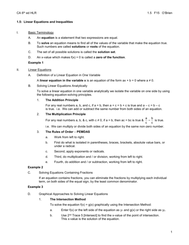
1.5 F15 O’Brien
CA 6th ed HLR
1.5: Linear Equations and Inequalities
I.
Basic Terminology
A.
An equation is a statement that two expressions are equal.
B.
To solve an equation means to find all of the values of the variable that make the equation true.
Such numbers are called solutions or roots of the equation.
C.
The set of all possible solutions is called the solution set.
D.
An x-value which makes f(x) = 0 is called a zero of the function.
Example 1
II.
Linear Equations
A.
Definition of a Linear Equation in One Variable
A linear equation in the variable x is an equation of the form ax + b = 0 where a ≠ 0.
B.
Solving Linear Equations Analytically
To solve a linear equation in one variable analytically we isolate the variable on one side by using
the following equation-solving principles.
1.
The Addition Principle
For any real numbers a, b, and c, if a = b, then a + c = b + c is true and a – c = b – c
is true. i.e. We can add or subtract the same number from both sides of an equation.
2.
The Multiplication Principle
a b

is true.
c c
i.e. We can multiply or divide both sides of an equation by the same non-zero number.
For any real numbers a, b, & c, with c ≠ 0, if a = b, then ac = bc is true &
3.
The Rules of Order – PEMDAS
a.
Work from left to right.
b.
First do what is isolated in parentheses, braces, brackets, absolute value bars, or
under a radical.
c.
Second, apply exponents or radicals.
d.
Third, do multiplication and / or division, working from left to right.
e.
Fourth, do addition and / or subtraction, working from left to right.
Example 2
C.
Solving Equations Containing Fractions
If an equation contains fractions, you can eliminate the fractions by multiplying each individual
term, on both sides of the equal sign, by the least common denominator.
Example 3
D.
Graphical Approaches to Solving Linear Equations
1.
The Intersection Method
To solve the equation f(x) = g(x) graphically using the Intersection Method:
a.
Enter f(x) or the left side of the equation as y1 and g(x) or the right side as y2.
b.
Use 2nd Trace 5 [Intersect] to find the x-value of the point of intersection.
This x-value is the solution of the equation.
1
1.5 F15 O’Brien
CA 6th ed HLR
2.
Possible Solutions
a.
One solution: the two lines intersect in one point.
b.
No solution: the two lines are parallel.
c.
Infinite solutions: the two lines coincide.
Example 4
3.
The x-Intercept or Zero Method
To solve the equation f(x) = g(x) graphically using the x-Intercept or Zero Method:
a.
At y1, enter f(x) – g(x).
b.
Use 2nd Trace 2 [Zero] to find the x-value of the x-intercept.
Note:
The x-value of the x-intercept of the graph of f(x)
= the zero of the function f(x)
= the solution of the equation f(x) = 0.
Example 5
III.
Types of Equations
A.
Conditional Equations
A conditional equation is true for only one specific value of x.
For example, x + 3 = 5 is only true when x = 2.
B.
Contradictions
A contradiction is an equation which is never true. It has no solutions.
For example, with the equation x = x + 1 if we subtract x from each side we get 0 = 1 which is
never true. Thus the equation x = x + 1 has no solution. The solution set of a contradiction is the
empty set or null set, denoted 0 .
C.
Identities
An identity is an equation which is always true. It has infinite solutions.
For example, the equation x + 6 = x + 2 + 4 is true for all possible values of x, so its solution is
the set of all real numbers,  ,   .
Example 6
IV.
Linear Inequalities in One Variable
A.
Definition
A linear inequality in one variable is an inequality that can be written in one of the following
forms, where a  0.
ax + b > 0
B.
ax + b < 0
ax  b  0
ax  b  0
Solving Linear Inequalities Analytically
To solve an inequality in one variable analytically, we isolate the variable on one side by using the
following properties of inequality.
For real numbers a, b, and c,
1.
If a < b, then a + c < b + c and a – c < b – c.
2.
i.e., The same number may be added to or subtracted from both sides of an inequality
without changing the solution set.
a b
 .
If c > 0 and a < b, then ac < bc and
c c
i.e. Each side of an inequality may be multiplied or divided by the same positive number
without changing the solution set.
2
1.5 F15 O’Brien
CA 6th ed HLR
3.
If c < 0 and a < b, ac > bc and
a b
 .
c c
i.e., When we multiply or divide both sides of an inequality by a negative number, the
direction of the inequality is reversed.
Note:
Similar properties exist for >,  , and  .
Example 7
C.
Solving Linear Inequalities Graphically
1.
The Intersection Method
To solve the inequality f(x) < g(x) or f(x) > g(x) graphically using the Intersection Method:
a.
Enter f(x) or the left side of the equation as y1 and g(x) or the right side as y2.
b.
Use 2nd Trace 5 [Intersect] to find the x-value of the point of intersection.
The solution set of f(x) < g(x) is the set of all real numbers x such that the
graph of f is below the graph of g.
The solution set of f(x) > g(x) is the set of all real numbers x such that the
graph of f is above the graph of g.
Note:
If the inequality symbol is  or  , the solution set includes the end value of the
interval, the x-value of the point of intersection.
Example 8
2.
The x-Intercept or Zero Method
To solve the inequality f(x) < g(x) or f(x) > g(x) graphically using the x-Intercept or
Zero Method:
a.
At y1, enter f(x) – g(x).
b.
Use 2nd Trace 2 [Zero] to find the x-value of the x-intercept.
The solution set of f(x) – g(x) < 0 is the set of all real numbers such that the
graph of f(x) – g(x) is below the x-axis.
The solution set of f(x) – g(x) > 0 is the set of all real numbers such that the
graph of f(x) – g(x) is above the x-axis.
Example 9
3
CA 6th ed HLR
1.5 F15 O’Brien
4
CA 6th ed HLR
1.5 F15 O’Brien
5
CA 6th ed HLR
1.5 F15 O’Brien
6
CA 6th ed HLR
1.5 F15 O’Brien
7