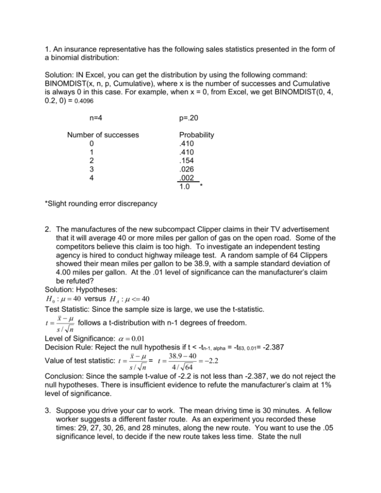
1. An insurance representative has the following sales statistics presented in the form of
a binomial distribution:
Solution: IN Excel, you can get the distribution by using the following command:
BINOMDIST(x, n, p, Cumulative), where x is the number of successes and Cumulative
is always 0 in this case. For example, when x = 0, from Excel, we get BINOMDIST(0, 4,
0.2, 0) = 0.4096
n=4
Number of successes
0
1
2
3
4
p=.20
Probability
.410
.410
.154
.026
.002
1.0 *
*Slight rounding error discrepancy
2. The manufactures of the new subcompact Clipper claims in their TV advertisement
that it will average 40 or more miles per gallon of gas on the open road. Some of the
competitors believe this claim is too high. To investigate an independent testing
agency is hired to conduct highway mileage test. A random sample of 64 Clippers
showed their mean miles per gallon to be 38.9, with a sample standard deviation of
4.00 miles per gallon. At the .01 level of significance can the manufacturer’s claim
be refuted?
Solution: Hypotheses:
H 0 :   40 versus H A :   40
Test Statistic: Since the sample size is large, we use the t-statistic.

x
follows a t-distribution with n-1 degrees of freedom.
t
s/ n
Level of Significance:   0.01
Decision Rule: Reject the null hypothesis if t < -tn-1, alpha = -t63, 0.01= -2.387

38.9  40
x
Value of test statistic: t 
= t
 2.2
4 / 64
s/ n
Conclusion: Since the sample t-value of -2.2 is not less than -2.387, we do not reject the
null hypotheses. There is insufficient evidence to refute the manufacturer’s claim at 1%
level of significance.
3. Suppose you drive your car to work. The mean driving time is 30 minutes. A fellow
worker suggests a different faster route. As an experiment you recorded these
times: 29, 27, 30, 26, and 28 minutes, along the new route. You want to use the .05
significance level, to decide if the new route takes less time. State the null
hypothesis, the alternative hypothesis, and the degrees of freedom in this test. What
is the critical value of the test statistic? Determine the mean and standard deviation
of the sample and use the test statistic to determine if you accept or reject the null
hypothesis.
Solution: Hypotheses:
H 0 :   30 min utes versus H A :   30 min utes
Test Statistic: Since the population standard deviation is unknown, we use the t-statistic.

x
follows a t-distribution with n-1 degrees of freedom.
t
s/ n
Level of Significance:   0.05
Decision Rule: Reject the null hypothesis if t < -tn-1, alpha = -t4, 0.05 = -2.132
Calculations:
Mean =
Stdev =
29
27
30
26
28
28
1.581139
Value of test statistic: t 

x
= t
28  30
 2.829
1.5811 / 5
s/ n
Conclusion: Since the sample t-value of -2.829 is less than the critical t-value of -2.132,
we reject the null hypotheses. There is sufficient evidence to conclude at 5% level of
significance that the alternative route is faster.
2. Teledko Associates is a marketing research firm that specializes in comparative
shopping. Teledko is hired by General Motors to compare the selling price of the
Pontiac Sunbird with the Chevy Cavalier. Posing as a potential customer, a
representative of Teledko visited 8 Pontiac dealerships in Metro City and 6 Chevrolet
dealerships in the same city and obtained quotes on comparable cars. The standard
deviation for the selling price of the 8 Pontiac Sunbirds is $350 and on the six
Cavaliers, $290. At the .02 level of significance is there a difference in the variation
of the quotes of the Sunbirds and the Cavaliers?
Solution: Hypotheses:
H0 :
 12
 12

1
H
:
1
versus
A
 22
 22
Test Statistic: We use the F-statistic F =
s12
with n1-1 and n2-1 degrees of freedom
s 22
Level of Significance:   0.02
Decision Rule: Reject the null hypothesis if F  F / 2,n11,n 21  F0.01, 7 ,5  10.45555
s12 350 2
Value of test statistic: F  2 
 1.4566
s 2 290 2
Conclusion: Since the sample F-value of 1.4566 is not greater than critical F-value of 10.4555, we do not reject the null hypotheses. There is insufficient evidence to conclude
at 2% level of significance that there exists a difference in the variation of the quotes of
the Sunbirds and the Cavaliers.
5. The owner of a mail-order catalog would like to compare her sales with the
geographic distribution of the population. According to the United States Bureau of the
Census, 21 percent of the population lives in the Northeast, 24 percent in the Midwest,
35 percent in the South, and 20 percent in the West. Listed below is a breakdown of a
sample of 400 orders randomly selected from those who shopped last month. At the
.01 significance level, does the distribution of the orders reflect the population?
Region
Frequency
Northeast
68
Midwest
104
South
155
West
73
Total
400
Solution: This is a problem of Chi-Squared test of goodness of fit.
Hypotheses:
H 0 : The percentages of the shopping populations are as listed according to the United
States Bureau of Census, versus
H A : At least two of the percentages are different.
Test Statistic: We use the  2 -statistic
4
 
2
Oi  ei 2
ei
Level of Significance:   0.01
Decision Rule: Reject the null hypothesis if  2   2  ,n1 =  2 0.01,3 = 11.34488
Value of test statistic: We construct the following table:
i 1
k
1
2
3
4
Sums:
Obsd. Freq.
68
104
155
73
400
Sample  2  0.0148348
Oi
0.17
0.26
0.3875
0.1825
1
ei
0.21
0.24
0.35
0.2
1
Oi-ei
-0.04
0.02
0.0375
-0.0175
(Oi-ei)^2
0.0016
0.0004
0.001406
0.000306
(Oi-ei)^2/ei
0.007619
0.0016667
0.0040179
0.0015313
0.0148348
Conclusion: Since the sample  2 -value of 0.0148348 is not greater than critical  2 value of 11.34488, we do not reject the null hypotheses. Thus we can conclude that at
1% level of significance, the distribution of the orders indeed reflects the population.