Kruskal-Wallis ANOVA with SPSS
Dr. Hussam El-Gayar of the Urology & Nephrology Center at Mansoura
University in Egypt found my SPSS lessons and asked me a question about the
analysis of some of his data. He wanted to compare six independent groups. His
criterion variable is continuously distributed. He had already conducted a one-way
parametric ANOVA with pairwise comparisons. I took a peek at the results of that
analysis and at the raw data and became concerned that both the homogeneity of
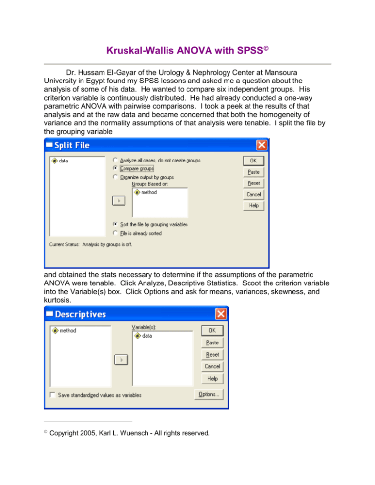
variance and the normality assumptions of that analysis were tenable. I split the file by
the grouping variable
and obtained the stats necessary to determine if the assumptions of the parametric
ANOVA were tenable. Click Analyze, Descriptive Statistics. Scoot the criterion variable
into the Variable(s) box. Click Options and ask for means, variances, skewness, and
kurtosis.

Copyright 2005, Karl L. Wuensch - All rights reserved.
2
De scri ptive Statistics
METHOD
1.00
2.00
3.00
4.00
5.00
6.00
DATA
Valid N
DATA
Valid N
DATA
Valid N
DATA
Valid N
DATA
Valid N
DATA
Valid N
(lis twis e)
(lis twis e)
(lis twis e)
(lis twis e)
(lis twis e)
(lis twis e)
N
St atist ic
97
97
97
97
97
97
97
97
97
97
97
97
Mean
St atist ic
39.8828
Variance
St atist ic
95.739
Sk ewness
St atist ic
St d. Error
-.448
.245
Kurtos is
St atist ic
St d. Error
2.212
.485
20.5936
33.483
-.207
.245
1.539
.485
28.0316
98.510
2.390
.245
16.615
.485
73.0409
4266.446
1.128
.245
1.625
.485
.8536
.484
2.827
.245
10.195
.485
129.4064
1606.246
.005
.245
-1. 178
.485
As you can see, there is both great heterogeneity of variance and, in some but
not all groups, great skewness. In this case, a nonparametric analysis is indicated. An
appropriate omnibus analysis is the Kruskal-Wallis ANOVA. To conduct it, click
Analyze, Nonparametrics, K Independent Samples. Scoot the criterion variable in the
Test Variable List and the grouping variable into the Grouping Variable box. Click
Define Range and identify the lowest and highest numeric values for the grouping
variable:
3
Click OK. The output includes mean ranks for each group:
Ranks
DATA
METHOD
1.00
2.00
3.00
4.00
5.00
6.00
Total
N
97
97
97
97
97
97
582
Mean Rank
358.90
198.29
269.71
359.47
49.87
512.77
Since our p value is less than the .05 criterion of statistical significance, we
conclude that there are significant differences among the groups.
Test Statisticsa,b
Chi-Square
df
As ymp. Sig.
DATA
431.651
5
.000
a. Kruskal Wallis Test
b. Grouping Variable: METHOD
We still do not know which groups differ significantly from which other groups, so
we continue on, comparing each group with each other group. If we make all possible
pairwise comparisons, we make 15 comparisons: Group 1 with 2, 3, 4, 5, and 6; Group
2 with 3, 4, 5, and 6; Group 3 with 4, 5, and 6; Group 4 with 5 and 6; and Group 5 with
6.
4
The Mann-Whitney U test is appropriate for comparing two independent groups.
Click Analyze, Nonparametric Tests, 2 Independent Samples. Scoot the criterion
variable into the Test Variable List and the grouping variable into the Grouping Variable
box. Click Define Groups and give the group numbers for the two groups to be
compared. Here I have asked to compare group 1 with group 6:
Click OK. The output includes for each group the mean rank and sum of ranks.
Both the Mann-Whitney and the Wilcoxon Rank Sum statistics are given. These two
statistics are equivalent, yielding the same p value. Since our p value is less than the
.05 criterion of statistical significance, we conclude that methods 1 and 6 differ from
each other significantly.
Ranks
DATA
METHOD
1.00
6.00
Total
N
97
97
194
Test Statisticsa
Mann-Whitney U
Wilcoxon W
Z
As ymp. Sig. (2-tailed)
DATA
9.000
4762.000
-12.089
.000
a. Grouping Variable: METHOD
Mean Rank
49.09
145.91
Sum of Ranks
4762.00
14153.00
5
Having illustrated how to compare two groups, I left to Dr. El-Gayar the task of
making the remaining 14 pairwise comparisons.
One final comment: Since some of the groups are greatly skewed, it is a good
idea to report medians rather than, or in addition to, means. SPSS Descriptives does
not compute medians, but SPSS Frequencies does. Here is how to do it: First, split the
file by the grouping method. Then click Analyze, Descriptive Statistics, Frequencies.
Select the criterion variable and click Statistics. Check Median and click Continue.
Click Format and check Suppress Tables With More Than ___ Categories. Enter the
number 2 in the categories box and click Continue.
6
Click OK. The output includes the median for each group:
Statistics
DA TA
1.00
N
2.00
Median
N
3.00
Median
N
4.00
Median
N
5.00
Median
N
6.00
Median
N
Valid
Missing
Median
Valid
Missing
Valid
Missing
Valid
Missing
Valid
Missing
Valid
Missing
97
0
39.8800
97
0
22.0000
97
0
30.0062
97
0
65.2500
97
0
.6704
97
0
131.8400
Copyright 2005, Karl L. Wuensch - All rights reserved.