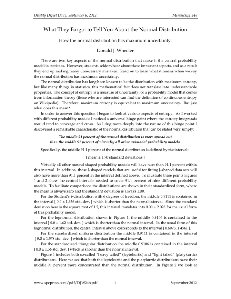
Quality Digest Daily, September 6, 2012
Manuscript 246
What They Forgot to Tell You About the Normal Distribution
How the normal distribution has maximum uncertainty.
Donald J. Wheeler
There are two key aspects of the normal distribution that make it the central probability
model in statistics. However, students seldom hear about these important aspects, and as a result
they end up making many unnecessary mistakes. Read on to learn what it means when we say
the normal distribution has maximum uncertainty.
The normal distribution has long been known to be the distribution with maximum entropy,
but like many things in statistics, this mathematical fact does not translate into understandable
properties. The concept of entropy is a measure of uncertainty for a probability model that comes
from information theory (those who are interested can find the definition of continuous entropy
on Wikipedia). Therefore, maximum entropy is equivalent to maximum uncertainty. But just
what does this mean?
In order to answer this question I began to look at various aspects of entropy. As I worked
with different probability models I noticed a universal hinge point where the entropy integrands
would tend to converge and cross. As I dug more deeply into the nature of this hinge point I
discovered a remarkable characteristic of the normal distribution that can be stated very simply:
The middle 91 percent of the normal distribution is more spread out
than the middle 91 percent of virtually all other unimodal probability models.
Specifically, the middle 91.1 percent of the normal distribution is defined by the interval:
[ mean ± 1.70 standard deviations ]
Virtually all other mound-shaped probability models will have more than 91.1 percent within
this interval. In addition, those J-shaped models that are useful for fitting J-shaped data sets will
also have more than 91.1 percent in the interval defined above. To illustrate these points Figures
1 and 2 show the central intervals needed to cover 91.1 percent of nine different probability
models. To facilitate comparisons the distributions are shown in their standardized form, where
the mean is always zero and the standard deviation is always 1.00.
For the Student’s t-distribution with 6 degrees of freedom, the middle 0.9111 is contained in
the interval [ 0.0 ± 1.656 std. dev. ] which is shorter than the normal interval. Since the standard
deviation here is the square root of 1.5, this interval translates into 0.00 ± 2.028 for the usual form
of this probability model.
For the lognormal distribution shown in Figure 1, the middle 0.9106 is contained in the
interval [ 0.0 ± 1.62 std. dev. ] which is shorter than the normal interval. In the usual form of this
lognormal distribution, the central interval above corresponds to the interval [ 0.6073, 1.4561 ].
For the standardized uniform distribution the middle 0.9111 is contained in the interval
[ 0.0 ± 1.578 std. dev. ] which is shorter than the normal interval.
For the standardized triangular distribution the middle 0.9106 is contained in the interval
[ 0.0 ± 1.56 std. dev. ] which is shorter than the normal interval.
Figure 1 includes both so-called “heavy tailed” (leptokurtic) and “light tailed” (platykurtic)
distributions. Here we see that both the leptokurtic and the platykurtic distributions have their
middle 91 percent more concentrated than the normal distribution. In Figure 2 we look at
www.spcpress.com/pdf/DJW246.pdf
1
September 2012
Donald J. Wheeler
What They Forgot to Tell You About the Normal Distribution
leptokurtic distributions having kurtosis values of 6.00, 8,90, 9.00, and 113.9 respectively.
Normal
skewness = 0.00
kurtosis = 3.00
-3
± 1.70
0.9109
-2
-1
0
1
2
3
Student's t-Dist.
with 6 d.f.
skewness = 0.00
kurtosis = 6.00
–4
–3
± 1.656
0.9111
–2
–1
0
1
2
3
4
3
4
LogNormal
E(lnX) = 0, SD(lnX) = 0.25
skewness(X) = 0.78
kurtosis(X) = 4.096
-3
± 1.62
0.9106
-2
-1
0
1
2
Uniform
skewness = 0.00
kurtosis = 1.80
-3
± 1.578
0.9111
-2
-1
0
1
2
3
Triangular
skewness = 0.57
kurtosis = 2.40
-3
± 1.56
0.9106
-2
-1
0
1
2
3
Figure 1: Central Intervals Needed to Cover 91.1% for Five Distributions
For the chi-square distribution with 4 degrees of freedom the middle 0.9111 is contained in
the interval [ 0.0 ± 1.44 std. dev. ] which is shorter than the normal interval. In the usual form for
this distribution this interval is [ 0.000, 8.073 ].
For the first lognormal distribution shown in Figure 2, the middle 0.9108 is contained in the
interval [ 0 ± 1.42 std. dev. ] which is shorter than the normal interval. In the usual form of this
lognormal distribution, the central interval shown corresponds to the interval [ 0.2756, 1.9907 ].
For the standardized exponential distribution the middle 0.9111 is contained within the
interval [ 0.0 ± 1.42 std. dev. ] which is shorter than the normal interval. In the usual form for this
distribution with mean = 1 the central interval above corresponds to the interval [ 0.000, 2.420 ].
For the second lognormal distribution shown in Figure 2, the middle 0.9113 is contained in
the interval [ 0 ± 1.02 std. dev. ] which is shorter than the normal interval. In the usual form of
this distribution, the central interval shown corresponds to the interval [ 0.000, 3.853 ].
We will look at a wider selection of probability models later, but this should suffice to
illustrate the earlier assertion. The middle 91 percent of the normal distribution is more spread
www.spcpress.com/pdf/DJW246.pdf
2
September 2012
Donald J. Wheeler
What They Forgot to Tell You About the Normal Distribution
out than the middle 91 percent of other probability models.
Chi-Square
± 1.44
0.9111
-2
-1
0
with 4 d.f.
skewness = 1.414
kurtosis = 6.00
1
2
3
4
LogNormal
Mean(lnX) = 0
SD(lnX) = 0.50
skewness(X) = 1.75
kurtosis(X) = 8.90
± 1.42
0.9108
-2
-1
0
1
2
3
4
5
Exponential
0.9111
-2
-1
0
skewness = 2.00
kurtosis = 9.00
± 1.42
1
2
3
4
5
LogNormal
Mean(lnX) = 0
SD(lnX) = 1.00
skewness(X) = 6.18
kurtosis(X) = 133.9
± 1.02
0.9113
-2
-1
0
1
2
3
4
5
Figure 2: 91.1% Central Intervals for Four “Heavy-Tailed” Distributions
TAIL-AREA PROBABILITIES
Looking at this in terms of tail-area probabilities, the normal distribution will have 8.9
percent of its area outside the interval [ mean ± 1.70 std. dev. ]. Virtually all other unimodal
probability models will have less than 8.9 percent outside this interval.
www.spcpress.com/pdf/DJW246.pdf
3
September 2012
Donald J. Wheeler
What They Forgot to Tell You About the Normal Distribution
The outer 9 percent of a normal distribution is further from the mean
than the outer 9 percent of virtually all other unimodal probability models.
It is customary to refer to the “tails” of a probability model as those regions that are outside
the interval defined by [ mean ± 1.00 std. dev. ]. However , if we define the “outer tails” to be
those regions that are outside [ mean ± 1.70 std. dev. ], then we can say that the normal distribution
has outer tails that are heavier than those of virtually all other unimodal probability models.
Normal
skewness = 0.00
kurtosis = 3.00
-3
-2
0.0891
Mean ±1.7 Std. Dev.
-1
0
1
2
3
Student's t-Dist.
with 6 d.f.
skewness = 0.00
kurtosis = 6.00
–4
–3
–2
0.0825
–1
0
1
2
3
4
3
4
LogNormal
E(lnX) = 0, SD(lnX) = 0.25
skewness(X) = 0.78
kurtosis(X) = 4.096
-3
-2
0.0757
-1
0
1
2
Uniform
skewness = 0.00
kurtosis = 1.80
-3
-2
0.0185
-1
0
1
2
3
Triangular
skewness = 0.57
kurtosis = 2.40
-3
-2
0.0707
-1
0
1
2
3
Figure 3: Outer Tail Areas for Five Standardized Distributions
The Student’s t-distribution with 6 degrees of freedom has an outer tail area of 8.25 percent,
which is less than that of the normal distribution. The lognormal distribution in Figure 3 has an
outer tail area of 7.57 percent, which is less than that of the normal distribution. The uniform
distribution has an outer tail area of 1.85 percent, which is less than that of the normal
distribution. The triangular distribution has an outer tail area of 7.07 percent, which is less than
that of the normal distribution.
The chi-square distribution with 4 d.f. has an outer tail area of 6.61 percent, which is less than
that of the normal distribution. The first lognormal distribution in Figure 4 has an outer tail area
www.spcpress.com/pdf/DJW246.pdf
4
September 2012
Donald J. Wheeler
What They Forgot to Tell You About the Normal Distribution
of 6.18 percent, which is less than that of the normal distribution. The exponential distribution
has an outer tail area of 6.72 percent, which is less than that of the normal distribution. And the
last lognormal distribution has an outer tail area of 4.73 percent, which is less than that of the
normal distribution.
Chi-Square
0.0661
Mean ±1.7 Std. Dev.
-2
-1
0
1
2
with 4 d.f.
skewness = 1.414
kurtosis = 6.00
3
4
LogNormal
0.0618
Mean(lnX) = 0
SD(lnX) = 0.50
skewness(X) = 1.75
kurtosis(X) = 8.90
-2
-1
0
1
2
3
4
5
Exponential
0.0672
-2
-1
0
1
2
skewness = 2.00
kurtosis = 9.00
3
4
5
LogNormal
0.0473
-2
-1
0
1
2
Mean(lnX) = 0
SD(lnX) = 1.00
skewness(X) = 6.18
kurtosis(X) = 133.9
3
4
5
Figure 4: Outer Tail Areas for Four “Heavy-Tailed” Distributions
While it may be no surprise that the outer tails of a normal are heavier than those of a
uniform distribution or a triangular distribution, it is a surprise that the outer tails of a normal are
heavier than those of the six “heavy-tailed” distributions shown in Figures 3 and 4. This is
www.spcpress.com/pdf/DJW246.pdf
5
September 2012
Donald J. Wheeler
What They Forgot to Tell You About the Normal Distribution
contrary to everything we teach. It is contrary to how we think. It is contrary to how we talk.
Yet this fact of life regarding probability models is not a matter of opinion. It can be verified by
anyone who is willing and capable of doing the computations.
Thus, the normal distribution is the distribution of maximum uncertainty. It has the most
diffuse middle 91%, and its outer tails are heavier than those of virtually any other moundshaped or useful J-shaped distribution. (This represents a paradigm shift for most of us,
including this author. So, if you are not feeling dizzy yet, you just don’t understand what you
have just read.) Referring to distributions with a large kurtosis as “heavy-tailed” distributions is
both misleading and inappropriate. As will be shown, most distributions have light outer tails
relative to the normal distribution!
FURTHER COMPARISONS
While the eight non-normal distributions shown above are illustrative, they hardly constitute
a rigorous argument that the normal distribution has outer tails that are as heavy as possible. For
those who seek a more thorough explanation I offer the following.
Figure 5 shows how the outer tail areas of the family of Student’s t-distributions compare to
the outer tail area of the normal distribution. In the usual way of drawing these distributions it is
the models having 3 through 10 degrees of freedom that appear to be heavy tailed. However, as
the degrees of freedom increase from 3 to 30, the outer tail areas increase towards the normal
value from below.
0.0900
Normal Outer Tail Area
0.0800
0.0700
Outer Tail Areas for
Student's t-distributions
0.0600
5
10
15
20
25
30 d.f.
Figure 5: Outer Tail Areas for Student’s t-Distributions
Figure 6 shows how the outer tail areas of the family of chi-square distributions compare to
the outer tail area of the normal distribution. Once again, it is those models with the small
number of degrees of freedom that are commonly thought of as being heavy-tailed. However, as
the degrees of freedom increase from 1 to 60 the outer tail areas start off small and eventually
increase towards the normal value from below.
www.spcpress.com/pdf/DJW246.pdf
6
September 2012
Donald J. Wheeler
What They Forgot to Tell You About the Normal Distribution
0.0900
Normal Outer Tail Area
0.0800
0.0700
Outer Tail Areas for
Chi Square distributions
0.0600
2
10
20
30
40
50
60 d.f.
Figure 6: Outer Tail Areas for Chi-Square Distributions
Figure 7 shows how the outer tail areas of the family of Log Normal distributions compare to
the outer tail area of the normal distribution. As the standard deviation of log X increases from
0.025 to 1.000 the outer tail areas decrease.
0.0900
Normal Outer Tail Area
0.0800
0.0700
0.0600
Outer Tail Areas for
Log Normal Distributions
0.0500
SD( ln X )
0.10
0.20
0.30
0.40
0.50
0.60
0.70
0.80
0.90
1.00
Figure 7: Outer Tail Areas for Log Normal Distributions
Figure 8 shows how the outer tail areas of the family of Weibull distributions compare to the
outer tail area of the normal distribution. Here the beta parameter is held constant at 1.00. As the
alpha parameter increases from 1.0 to 4.5 the Weibull distribution will first approach and then
recede from the normal distribution. During this period of closest approach the Weibull outer tail
areas briefly exceed the normal value of 0.0891.
The Weibull distributions with heavier than normal outer tail areas have skewness values
ranging from 0.05 to -0.13 and kurtosis values ranging from 2.71 to 2.77. Their outer tail areas
range up to 0.0898, which exceeds the normal value by less than one percent. Since such small
www.spcpress.com/pdf/DJW246.pdf
7
September 2012
Donald J. Wheeler
What They Forgot to Tell You About the Normal Distribution
differences simply do not show up in practice, we have to consider these outer tail areas to be
equivalent to those of the normal distribution.
0.0900
Normal Outer Tail Area
skewness = -0.13
kurtosis = 2.77
0.0800
skewness = 0.05
kurtosis = 2.71
0.0700
Outer Tail Areas for
Weibull Distributions
0.0600
1.0
1.5
Alpha Value
2.0
2.5
3.0
3.5
4.0
4.5
Figure 8: Outer Tail Areas for Weibull Distributions
Thus, we find that while the outer tail area of 0.0891 for the normal distribution is not an
absolute maximum, it appears to be so close to the maximum that it makes no practical
difference. To further investigate the question of what models might have heavier outer tails
than the normal I looked at an additional 3,266 mound-shaped and J-shaped probability models.
These models are shown in Figure 9 using the shape characterization plane. In the shape
characterization plane each probability model is represented by a point. The coordinates for the
point representing each probability model are the skewness squared (shown on the X axis) and
the kurtosis (shown on the Y axis) for that model. These 3,266 models were selected to obtain
uniform coverage of the regions shown in Figure 9.
In Figure 9 the Normal distribution is located at the point [ 0.00, 3.00 ]. The family of Log
Normal distributions is represented by the line labeled L. The line labeled W shows the family of
Weibull distributions, and the line labeled G shows the family of Gamma distributions, which
includes the family of chi-square distributions as a subset. The vertical black line labeled T shows
the family of Student’s t-distributions.
The 2,010 mound-shaped distributions shown in red consisted of 1,718 Burr distributions and
292 Beta distributions. These distributions have outer tail areas that range from 0.0573 to 0.0890,
and so all have lighter outer tails than a normal distribution.
The six white dots found directly above and below the normal distribution represent six
mound-shaped Burr distributions that have outer tail areas of 0.0892 to 0.0898. Thus, these six
mound shaped models have outer tails that are very slightly heavier than the normal. Once
again, since such small differences simply do not show up in practice, we have to consider these
outer tail areas to be equivalent to those of the normal distribution.
The 1250 J-shaped Beta distributions shown in purple in Figure 8 have outer tail areas that
range from 0.0665 to 0.0816. Thus, they all have lighter outer tails than the normal distribution.
(These 1250 Beta distributions all have end points that are at least six standard deviations
apart. J-shaped Beta distributions that span less than six standard deviations will have a
truncated upper tail and so will not provide useful models for fitting J-shaped histograms which
are logically one-sided.)
www.spcpress.com/pdf/DJW246.pdf
8
September 2012
Donald J. Wheeler
What They Forgot to Tell You About the Normal Distribution
Kurtosis
Skewness Squared
0
1
L
2
3
4
W
G
5
7
8
9
12
11
10
9
T
8
7
1250 J-Shaped Distributions
with Outer Tail Areas
That Are Less Than 0.0816
6
5
4
2010 Mound Shaped Distributions
with Outer Tail Areas
That Are Less Than 0.0890
3
2
Six Mound Shaped Distributions
with Outer Tail Areas
Between 0.0892 and 0.0898
1
Figure 9: Outer Tail Areas for 3266 Probability Models
Including the 164 models in Figures 1 through 8 we have, at this point, considered 3,430
probability models and have found only 15 models that have very slightly heavier outer tail areas
than the normal (6 Burrs and 9 Weibulls). The maximum outer tail area found was 0.0898. The
www.spcpress.com/pdf/DJW246.pdf
9
September 2012
Donald J. Wheeler
What They Forgot to Tell You About the Normal Distribution
normal outer tail area of 0.0891 is so close to this observed maximum that there is no practical
difference between these outer tail areas.
Therefore, based on the examination of over 3,400 probability models, it is safe to say that the
middle 91 percent of the normal distribution is essentially spread out to the maximum extent
possible, and its outer tails are as heavy or heavier than those of any mound-shaped or useful Jshaped distribution. When choosing a probability model, you simply will not find a useful
model with a central area that is more diffuse, or that has heavier outer tails, than the normal
distribution. This is what it means for the normal distribution to be the distribution of maximum
uncertainty.
SELECTING A PROBABILITY MODEL
One of the implications of the normal distribution having maximum entropy is the following:
If all you know about a distribution is the mean and the variance, then the probability model that
will impose the fewest constraints upon the situation will be a normal distribution having that
mean and variance.
In addition, maximum entropy also means that the use of any other probability model will
require additional information beyond the mean and the variance. Any time you fit a probability
model to your data you will need to have some basis for choosing the model you are using.
When you choose any model other than the normal you are making a dual determination: First,
that the middle 91% of the probability is more concentrated than in a normal, and second, that the
outer tails are lighter than in a normal distribution. Such determinations will have to be based
upon some sort of information. So let’s consider where such information may be found.
Can we get this information from the data? Once we have estimated the mean and the
variance we have essentially obtained all of the useful information that can be had from
numerical summaries of the data. As I showed in my column “Problems with Skewness and
Kurtosis, Part Two, Quality Digest Daily, Aug. 2, 2011, the skewness and kurtosis statistics are
essentially worthless. (There I showed that with 200 data, the skewness and kurtosis statistics
would not differentiate between a nearly normal distribution and an exponential distribution.)
So, trying to “fit a probability model” to your data using the “shape statistics” is simply going to
be an exercise in fitting a model to the noise within your data. Remember, we are talking about
constraining the probability model, and any such constraint must be based on knowledge rather
than speculation. If you are going to speculate, you should always use a worst-case approach,
and what I have just demonstrated in this paper is that the worst-case distribution is the normal
distribution. So, while we may do the computations and fit a non-normal model to the data
based on information from those data, such an exercise will usually be a triumph of computation
over reality, and the results will be, more often than not, an example of being misled by noise.
Can we get the needed information from the histogram? Often we have a skewed histogram,
but is a skewed histogram a signal that the probability model should be skewed? The most
common reason for a skewed histogram is an underlying process that is changing while the data
are being collected. As the process moves around, the data move with the process, and the
resulting pile of data tells us nothing about what probability model to use. The more skewed the
histogram, the more likely that the process is changing. Thus, until the data have been shown to
display a reasonable degree of homogeneity (i.e. statistical control), any attempt to use the shape
of the histogram to select a model to use will be undermined by the lack of homogeneity within
the data.
www.spcpress.com/pdf/DJW246.pdf
10
September 2012
Donald J. Wheeler
What They Forgot to Tell You About the Normal Distribution
“But what if I have a detectable lack-of-fit when I test for normality?” Every lack-of-fit test
makes an implicit assumption that the data are homogeneous. A detectable lack-of-fit will, in
most cases, be an indication of a lack of homogeneity rather than being a signal that you need
something other than a normal distribution as your model.
So, if we can’t use numerical summaries, and if we can’t use the histogram or tests of fit, how
can we ever determine what kind of probability model to use when fitting our data? Context will
sometimes offer a clue. If the data are known to be bounded on one side and if the data tend to
pile up against this boundary, then a skewed model might be appropriate. However, since any
attempt to fit a probability model to your data will require estimates of parameters for the
probability model, and since these estimates will only be reliable when the data are homogenous,
a preliminary step in fitting a model will be to demonstrate that your data display a reasonable
degree of homogeneity. And the only way to do this is to place the data on a process behavior
chart. Without the use of a process behavior chart, any attempt to use context to fit a probability
model to your data may be undermined by a lack of homogeneity within your data. (For an
example of this see my column “What is Leptokurtophobia?” Quality Digest Daily, August 1,
2012.)
While the software may tempt you to fit a non-normal probability model to your data,
information theory requires that you have more than the estimated values for the mean and
variance in order to do so. You cannot get this additional information from the data, you cannot
get this additional information from the histogram, and unless the data happen to be
homogeneous, you cannot successfully use information obtained from the context. Without the
necessary information required to constrain your probability model, your worst-case, maximum
entropy choice will be a normal distribution. The middle 91 percent will be dispersed to the
maximum extent possible, and the outer 9 percent will be further from the mean than the outer 9
percent of almost any other distribution.
FITTING MODELS AND SPC
The discussion above pertains to the all too common practice of fitting a model to the data.
Since this exercise is frequently done without having first qualified the data by checking them for
homogeneity, the results frequently end up being completely worthless. Moreover, any analysis
that is built upon such a fitted model is likely to end up being an exercise in futility.
“But I thought we had to fit a model to our data before we could place the data on a control
chart.” No, you don’t. While there are those who teach such nonsense, it is simply not true. It
never was true, and it will never be true. The fitting of a probability model prior to the use of a
process behavior chart is a heresy that has become popular with the rise of software. The
teachers of this heresy will often claim that “we could not easily fit models before we had
computers, and so we skipped this step in the past.” While the first part of this claim is true, the
last part about skipping this step in the past is completely false. When people do not understand
how SPC works, they tend to come up with novel, yet incorrect, ideas and explanations. (These
explanations are frequently like the child’s statement “The trees make the wind blow.” While all
the elements are there, they are not quite assembled correctly.)
So, let me be clear on this point which I learned from Ed Deming, who learned it from Walter
Shewhart, who invented the technique. There are no distributional assumptions imposed upon
the data, or otherwise required, for the use of either the average and range chart or the XmR
chart. In fact, a process cannot be said to be characterized by any probability model until it
displays a reasonable degree of predictability. To paraphrase Shewhart, the purpose of a process
www.spcpress.com/pdf/DJW246.pdf
11
September 2012
Donald J. Wheeler
What They Forgot to Tell You About the Normal Distribution
behavior chart is to determine if a probability model exists. It makes no assumptions about the functional
form of such a probability model.
The use of a process behavior chart is preliminary to the use of the traditional techniques of
statistics, all of which assume homogeneity for the data. If your understanding of SPC differs
from this, then you need to go back and study SPC more carefully using better sources.
If you have not qualified your data by putting them on a process behavior chart and finding
them to display a reasonable degree of homogeneity, then any attempt to fit a model to your data
is premature. And when you do try to fit a model, you will need strong evidence indeed to argue
for anything more specific than a normal distribution.
POSTSCRIPT
This article used a split of 91 percent and 9 percent between the central portion and the outer
tails. Subsequent research shows that equally strong arguments can be made for other splits
ranging from 88/12 to 92/8. Thus, if we define the cut-off for the outer tails anywhere between
1.55 sigma and 1.75 sigma we can still say that the outer tails of the normal distribution are
essentially as heavy as, or heavier than, the outer tails of any unimodal probability model.
www.spcpress.com/pdf/DJW246.pdf
12
September 2012