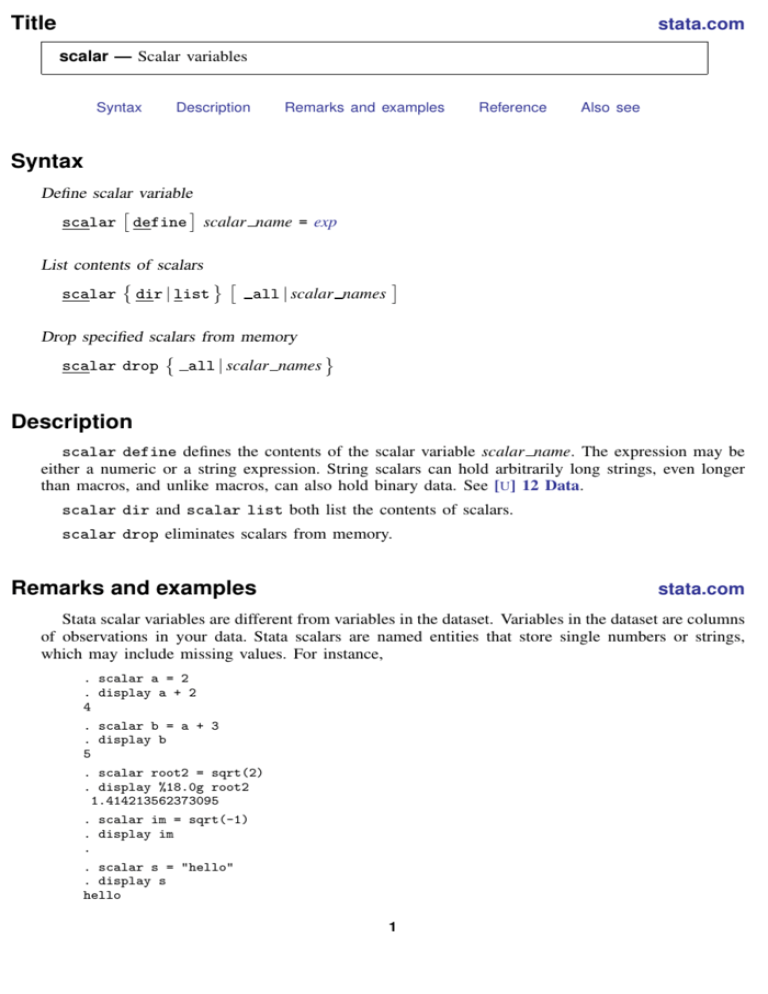
Title
stata.com
scalar — Scalar variables
Syntax
Description
Remarks and examples
Reference
Also see
Syntax
Define scalar variable
scalar define scalar name = exp
List contents of scalars
all | scalar names
scalar dir | list
Drop specified scalars from memory
scalar drop
all | scalar names
Description
scalar define defines the contents of the scalar variable scalar name. The expression may be
either a numeric or a string expression. String scalars can hold arbitrarily long strings, even longer
than macros, and unlike macros, can also hold binary data. See [U] 12 Data.
scalar dir and scalar list both list the contents of scalars.
scalar drop eliminates scalars from memory.
Remarks and examples
stata.com
Stata scalar variables are different from variables in the dataset. Variables in the dataset are columns
of observations in your data. Stata scalars are named entities that store single numbers or strings,
which may include missing values. For instance,
. scalar a = 2
. display a + 2
4
. scalar b = a + 3
. display b
5
. scalar root2 = sqrt(2)
. display %18.0g root2
1.414213562373095
. scalar im = sqrt(-1)
. display im
.
. scalar s = "hello"
. display s
hello
1
2
scalar — Scalar variables
scalar list can be used to display the contents of macros (as can display for reasons that
will be explained below), and scalar drop can be used to eliminate scalars from memory:
. scalar list
s = hello
im =
.
root2 = 1.4142136
b =
5
a =
2
. scalar list a b
a =
b =
2
5
. scalar drop a b
. scalar list
s = hello
im =
.
root2 = 1.4142136
. scalar drop _all
. scalar list
.
Although scalars can be used interactively, their real use is in programs. Stata has macros and scalars,
and deciding when to use which can be confusing.
Example 1
Let’s examine a problem where either macros or numeric scalars could be used in the solution.
There will be occasions in your programs where you need something that we will describe as a
mathematical scalar — one number. For instance, let’s assume that you are writing a program and
need the mean of some variable for use in a subsequent calculation. You can obtain the mean after
summarize from r(mean) (see Stored results in [R] summarize), but you must obtain it immediately
because the numbers stored in r() are reset almost every time you give a statistical command.
Let’s complicate the problem: to make some calculation, you need to calculate the difference in
the means of two variables, which we will call var1 and var2. One solution to your problem is to
use macros:
summarize var1, meanonly
local mean1 = r(mean)
summarize var2, meanonly
local mean2 = r(mean)
local diff = ‘mean1’ - ‘mean2’
Subsequently, you use ‘diff’ in your calculation. Let’s understand how this works. You summarize
var1, meanonly; including the meanonly option suppresses the output from the summarize command
and the calculation of the variance. You then store the contents of r(mean) — the just-calculated
mean — in the local macro mean1. You then summarize var2, again suppressing the output, and
save that just-stored result in the local macro mean2. Finally, you create another local macro called
diff, which contains the difference. In making this calculation, you must put the mean1 and mean2
local macro names in single quotes because you want the contents of the macros. If the mean of
var1 is 3 and the mean of var2 is 2, you want the numbers 3 and 2 substituted into the formula
for diff to produce 1. If you omitted the single quotes, Stata would think that you are referring
to the difference—not of the contents of macros named mean1 and mean2—but of two variables
named mean1 and mean2. Those variables probably do not exist, so Stata would then produce an
error message. In any case, you put the names in the single quotes.
scalar — Scalar variables
3
Now let’s consider the solution using Stata scalars:
summarize
scalar m1
summarize
scalar m2
scalar df
var1, meanonly
= r(mean)
var2, meanonly
= r(mean)
= m1 - m2
The program fragments are similar, although this time we did not put the names of the scalars used in
calculating the difference — which we called df this time — in single quotes. Stata scalars are allowed
only in expressions — they are a kind of variable — and Stata knows that you want the contents of
those variables.
So, which solution is better? There is certainly nothing to recommend one over the other in terms
of program length — both programs have the same number of lines and, in fact, there is a one-to-one
correspondence between what each line does. Nevertheless, the scalar-based solution is better, and
here is why:
Macros are printable representations of things. When we said local mean1 = r(mean), Stata took
the contents of r(mean), converted them into a printable form from its internal (and highly accurate)
binary representation, and stored that string of characters in the macro mean1. When we created
mean2, Stata did the same thing again. Then when we said local diff = ‘mean1’ - ‘mean2’, Stata
first substituted the contents of the macros mean1 and mean2 — which are really strings — into the
command. If the means of the two variables are 3 and 2, the printable string representations stored in
mean1 and mean2 are “3” and “2”. After substitution, Stata processed the command local diff = 3
- 2, converting the 3 and 2 back into internal binary representation to take the difference, producing
the number 1, which it then converted into the printable representation “1”, which it finally stored in
the macro diff.
All of this conversion from binary to printable representation and back again is a lot of work for
Stata. Moreover, although there are no accuracy issues with numbers like 3 and 2, if the first number
had been 3.67108239891 × 10−8 , there would have been. When converting to printable form, Stata
produces representations containing up to 17 digits and, if necessary, uses scientific notation. The
first number would have become 3.6710823989e-08, and the last digit would have been lost. In
computer scientific notation, 17 printable positions provides you with at least 13 significant digits.
This is a lot, but not as many as Stata carries internally.
Now let’s trace the execution of the solution by using scalars. scalar m1 = r(mean) quickly
copied the binary representation stored in r(mean) into the scalar m1. Similarly, executing scalar
m2 = r(mean) did the same thing, although it saved it in m2. Finally, scalar df = m1 - m2 took the
two binary representations, subtracted them, and copied the result to the scalar df. This produces a
more accurate result.
Naming scalars
Scalars can have the same names as variables in the data and Stata will not become confused.
You, however, may. Consider the following Stata command:
. generate newvar = alpha*beta
What does it mean? It certainly means to create a new data variable named newvar, but what will
be in newvar? There are four possibilities:
• Take the data variable alpha and the data variable beta, and multiply the corresponding observations
together.
• Take the scalar alpha and the data variable beta, and multiply each observation of beta by
alpha.
4
scalar — Scalar variables
• Take the data variable alpha and the scalar beta, and multiply each observation of alpha by
beta.
• Take the scalar alpha and the scalar beta, multiply them together, and store the result repeatedly
into newvar.
How Stata decides among these four possibilities is the topic of this section.
Stata’s first rule is that if there is only one alpha (a data variable or a scalar) and one beta (a
data variable or a scalar), Stata selects the one feasible solution and does it. If, however, there is
more than one alpha or more than one beta, Stata always selects the data-variable interpretation in
preference to the scalar.
Assume that you have a data variable called alpha and a scalar called beta:
. list
alpha
1.
2.
3.
1
3
5
. scalar list
beta =
3
. gen newvar = alpha*beta
. list
1.
2.
3.
alpha
newvar
1
3
5
3
9
15
The result was to take the data variable alpha and multiply it by the scalar beta. Now let’s start
again, but this time, assume that you have a data variable called alpha and both a data variable and
a scalar called beta:
. scalar list
beta =
3
. list
1.
2.
3.
alpha
beta
1
3
5
2
3
4
. gen newvar = alpha*beta
. list
1.
2.
3.
alpha
beta
newvar
1
3
5
2
3
4
2
9
20
scalar — Scalar variables
5
The result is to multiply the data variables, ignoring the scalar beta. In situations like this, you can
force Stata to use the scalar by specifying scalar(beta) rather than merely beta:
. gen newvar2 = alpha*scalar(beta)
. list
alpha
beta
newvar
newvar2
1
3
5
2
3
4
2
9
20
3
9
15
1.
2.
3.
The scalar() pseudofunction, placed around a name, says that the name is to be interpreted as the
name of a scalar, even if a data variable by the same name exists. You can use scalar() around
all your scalar names if you wish; there need not be a name conflict. Obviously, it will be easiest if
you give your data and scalars different names.
Technical note
The advice to name scalars and data variables differently may work interactively, but in programming
situations, you cannot know whether the name you have chosen for a scalar conflicts with the data
variables because the data are typically provided by the user and could have any names whatsoever.
One solution — and not a good one — is to place the scalar() pseudofunction around the names
of all your scalars when you use them. A much better solution is to obtain the names for your scalars
from Stata’s tempname facility; see [P] macro. There are other advantages as well. Let’s go back to
calculating the sum of the means of variables var1 and var2. Our original draft looked like
summarize
scalar m1
summarize
scalar m2
scalar df
var1, meanonly
= r(mean)
var2, meanonly
= r(mean)
= m1 - m2
A well-written draft would look like
tempname m1 m2 df
summarize var1, meanonly
scalar ‘m1’ = r(mean)
summarize var2, meanonly
scalar ‘m2’ = r(mean)
scalar ‘df’ = ‘m1’ - ‘m2’
We first declared the names of our temporary scalars. Actually, tempname creates three new local
macros named m1, m2, and df, and places in those macros names that Stata makes up, names that
are guaranteed to be different from the data. (m1, for your information, probably contains something
000001.) When we use the temporary names, we put single quotes around them — m1 is not
like
the name we want; we want the name that is stored in the local macro named m1.
That is, if we type
scalar m1 = r(mean)
then we create a scalar named m1. After tempname m1 m2 df, if we type
scalar ‘m1’ = r(mean)
then we create a scalar named with whatever name happens to be stored in m1. It is Stata’s responsibility
to make sure that name is valid and unique, and Stata did that when we issued the tempname command.
As programmers, we never need to know what is really stored in the macro m1; all we need to do is
put single quotes around the name whenever we use it.
6
scalar — Scalar variables
There is a second advantage to naming scalars with names obtained from tempname. Stata knows
that they are temporary — when our program concludes, all temporary scalars will be automatically
dropped from memory. And, if our program calls another program, that program will not accidentally
use one of our scalars, even if the programmer happened to use the same name. Consider
program myprog
( lines omitted )
tempname m1
scalar ‘m1’ = something
mysub
( lines omitted )
end
program mysub
( lines omitted )
tempname m1
scalar ‘m1’ = something else
( lines omitted )
end
Both myprog and mysub refer to a scalar, ‘m1’; myprog defines ‘m1’ and then calls mysub, and
mysub then defines ‘m1’ differently. When myprog regains control, however, ‘m1’ is just as it was
before myprog called mysub!
It is unchanged because the scalar is not named m1: it is named something returned by tempname — a
guaranteed unique name — and that name is stored in the local macro m1. When mysub is executed,
Stata safely hides all local macros, so the local macro m1 in mysub has no relation to the local macro
m1 in myprog. mysub now puts a temporary name in its local macro m1 — a different name because
tempname always returns unique names — and mysub now uses that different name. When mysub
completes, Stata discards the temporary scalars and macros and restores the definitions of the old
temporary macros, and myprog is off and running again.
Even if mysub had been poorly written in the sense of not obtaining its temporary names from
tempname, myprog would have no difficulty. The use of tempname by myprog is sufficient to
guarantee that no other program can harm it. For instance, pretend mysub looked like
program mysub
( lines omitted )
scalar m1 = something else
( lines omitted )
end
mysub is now directly using a scalar named m1. That will not interfere with myprog, however, because
myprog has no scalar named m1. Its scalar is named ‘m1’, a name obtained from tempname.
Technical note
One result of the above is that scalars are not automatically shared between programs. The scalar
‘m1’ in myprog is different from either of the scalars m1 or ‘m1’ in mysub. What if mysub needs
myprog’s ‘m1’?
One solution is not to use tempname: you could write myprog to use the scalar m1 and mysub to
use the scalar m1. Both will be accessing the same scalar. This, however, is not recommended.
scalar — Scalar variables
7
A better solution is to pass ‘m1’ as an argument. For instance,
program myprog
( lines omitted )
tempname m1
scalar ‘m1’ = something
mysub ‘m1’
( lines omitted )
end
program mysub
args m1
( lines omitted )
commands using ‘m1’
( lines omitted )
end
We passed the name of the scalar given to us by tempname — ‘m1’ — as the first argument to mysub.
mysub picked up its first argument and stored that in its own local macro by the same name — m1.
Actually, mysub could have stored the name in any macro name of its choosing; the line reading args
m1 could read args m2, as long as we changed the rest of mysub to use the name ‘m2’ wherever it
uses the name ‘m1’.
Reference
Kolev, G. I. 2006. Stata tip 31: Scalar or variable? The problem of ambiguous names. Stata Journal 6: 279–280.
Also see
[P] macro — Macro definition and manipulation
[P] matrix — Introduction to matrix commands
[U] 18.3 Macros
[U] 18.7.2 Temporary scalars and matrices