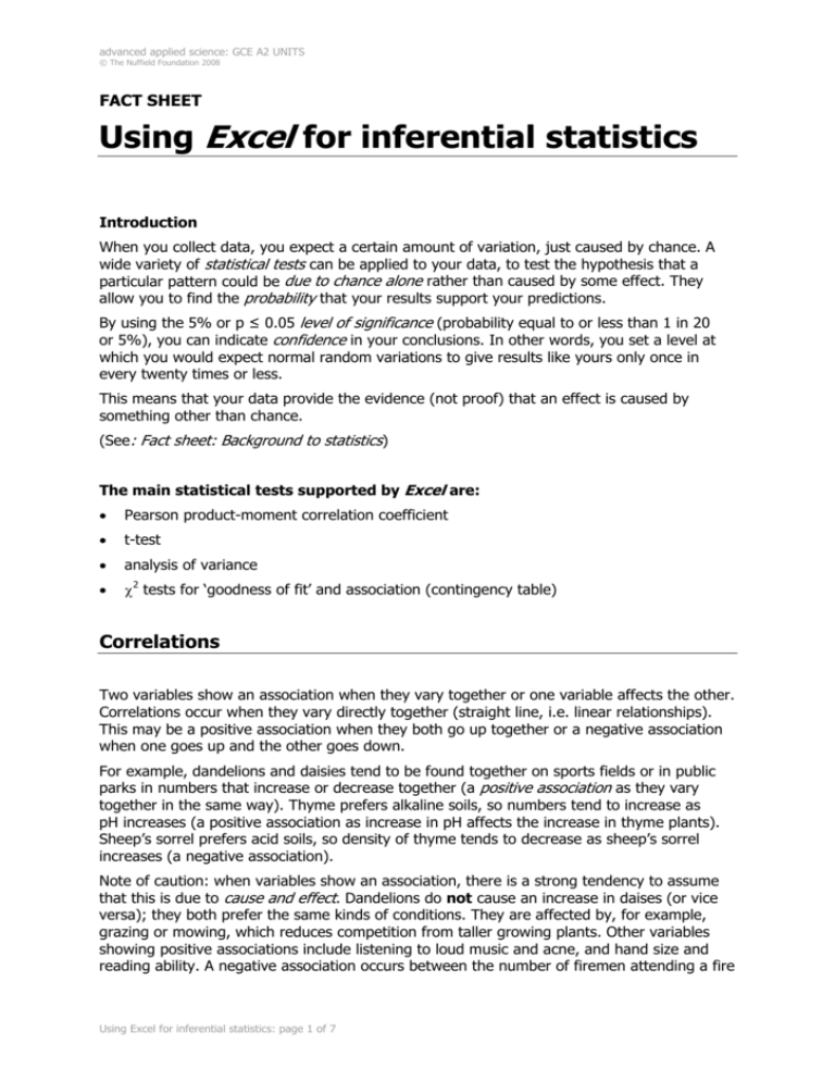
advanced applied science: GCE A2 UNITS
© The Nuffield Foundation 2008
FACT SHEET
Using Excel for inferential statistics
Introduction
When you collect data, you expect a certain amount of variation, just caused by chance. A
wide variety of statistical tests can be applied to your data, to test the hypothesis that a
particular pattern could be due to chance alone rather than caused by some effect. They
allow you to find the probability that your results support your predictions.
By using the 5% or p ≤ 0.05 level of significance (probability equal to or less than 1 in 20
or 5%), you can indicate confidence in your conclusions. In other words, you set a level at
which you would expect normal random variations to give results like yours only once in
every twenty times or less.
This means that your data provide the evidence (not proof) that an effect is caused by
something other than chance.
(See: Fact sheet: Background to statistics)
The main statistical tests supported by Excel are:
•
Pearson product-moment correlation coefficient
•
t-test
•
analysis of variance
•
χ2 tests for ‘goodness of fit’ and association (contingency table)
Correlations
Two variables show an association when they vary together or one variable affects the other.
Correlations occur when they vary directly together (straight line, i.e. linear relationships).
This may be a positive association when they both go up together or a negative association
when one goes up and the other goes down.
For example, dandelions and daisies tend to be found together on sports fields or in public
parks in numbers that increase or decrease together (a positive association as they vary
together in the same way). Thyme prefers alkaline soils, so numbers tend to increase as
pH increases (a positive association as increase in pH affects the increase in thyme plants).
Sheep’s sorrel prefers acid soils, so density of thyme tends to decrease as sheep’s sorrel
increases (a negative association).
Note of caution: when variables show an association, there is a strong tendency to assume
that this is due to cause and effect. Dandelions do not cause an increase in daises (or vice
versa); they both prefer the same kinds of conditions. They are affected by, for example,
grazing or mowing, which reduces competition from taller growing plants. Other variables
showing positive associations include listening to loud music and acne, and hand size and
reading ability. A negative association occurs between the number of firemen attending a fire
Using Excel for inferential statistics: page 1 of 7
advanced applied science: GCE A2 UNITS
© The Nuffield Foundation 2008
and the amount of losses in the fire; there is a negative association between mobile phone
use and sperm count. Can you suggest reasons for these associations?
Correlation coefficients
Correlation coefficients are statistical tests used to show the strength of an association. They
can be used to calculate the probability that data show an association (positive or negative)
by chance alone. Two commonly used tests for association are the Pearson product-moment
correlation coefficient (r) and the Spearman rank order correlation coefficient (ρ Greek letter
rho).
Pearson is used for parametric data, i.e. data that is normally distributed and Spearman for
non-parametric data that can be placed in order of magnitude (i.e. ranked). Excel has a
function to calculate the Pearson coefficient and can be modified to calculate Spearman.
In both cases, values vary between +1 and -1:
-1
0
+1
Perfect negative correlation
No correlation
Perfect positive correlation
Investigating correlations
Paired data are collected, so each value for one variable has an associated value for the
second variable. These can be used as coordinates to plot a scatter graph. The value of the
correlation coefficient depends on how closely data approximate to a straight line
relationship. Perfect correlations (+1 or -1) have plots that lie on a straight line:
r = +1
r = -1
Sometimes there is no correlation at all:
r=0
Using Excel for inferential statistics: page 2 of 7
r=0
advanced applied science: GCE A2 UNITS
© The Nuffield Foundation 2008
More often, it will be somewhere in between:
r = 0.49
r = - 0.71
How do you interpret correlation coefficient scores? For example, when comparing a score of
0.90 with 0.79? You use the probability of obtaining a score to decide whether the value is
significant or not.
You want to know if your data support the hypothesis that they show a significant
correlation. This is called the experimental or alternative hypothesis, HA. You can refine this
by testing either for a positive or a negative correlation:
e.g. HA = there is a significant positive association between the rate of water loss in woodlice
and the external temperature
Coefficients of correlation test the null hypothesis, H0, that there is no significant correlation,
any apparent correlation is due solely to chance.
In the case of the woodlice, H0 = there is no significant correlation between the rate of
water loss by woodlice and their external temperature, any apparent correlation is due solely
to chance.
The coefficient of correlation can be used to find the probability that the data support the
null hypothesis and this information can be used to support or reject the null hypothesis at a
pre-chosen level of significance, usually p ≤ 0.05:
ƒ
if you accept the null hypothesis, you reject the alternative hypothesis
ƒ
if you reject the null hypothesis, you the accept alternative hypothesis
Degrees of freedom
The number of values in a sample has an important effect. Imagine (or try) tossing a coin a
few times. Probability suggests that heads will occur half the time, but by chance you will
occasionally get, say, 5 heads in a row, or none. Keep going and the fluctuations caused by
chance tend to iron out. Runs of heads are matched by runs of tails.
Hence, every so often a small sample of results is quite likely to give a high value for a
correlation coefficient solely by chance, rather than because there is a genuine correlation.
Conversely, a large sample is much less likely to give a high value just due to chance alone.
Statistical tests use ‘degrees of freedom’ to take this effect into account. For Pearson’s r, the
degrees of freedom are found by subtracting 2 from the number of pairs of data (written as
df = N-2).
Using Excel for inferential statistics: page 3 of 7
advanced applied science: GCE A2 UNITS
© The Nuffield Foundation 2008
You also need to consider whether to use a one- or two-tailed test of significance. Pearson’s
correlation coefficient may give a positive value greater than zero (positive association) or a
negative value less than zero (negative association), i.e. it is usually used as a two-tailed
test. However, if you have a good theoretical reason for predicting a positive or negative
outcome (stated in your hypothesis), you can use it as a one-tailed test.
If you plot a scattergram, you can establish whether you want to test for a positive or a
negative correlation and use a one-tailed test of significance. If you have any doubts, use
the two-tailed test, you are less likely to make an error of finding a significant correlation
where none exists.
For a set of data with n paired values x and y, means x and y with standard deviations
and sy the Pearson correlation coefficient is:
sx
The longer second formula is actually easier to work out with a calculator!
Using Excel to calculate Pearson’s r
1
Type the paired data into two neighbouring columns on the spreadsheet.
2
Click to highlight the cell where the statistic will appear.
3
Format this cell to give 3 decimal places.
4
With the cell still highlighted, click fx next to the formula box, the Insert Function
dialogue box will appear.
5
Click the Select a category box to get the drop down menu and select Statistical.
6
Scroll down and select PEARSON.
7
Click OK to get the Function Arguments dialogue box.
8
Check that the cursor is flashing in Array1 (if not, click on the box).
9
Enter the data by clicking and dragging over the cells with the first set of data.
10 Click on the Array2 box and enter the second set of data (those paired with the first set).
11 Click OK to get the value for the Pearson r coefficient for these data. If Array1 or Array2
are empty or have a different number of data points, #N/A will appear.
Critical values
To check the r value for significance, you will need to find the number of degrees of freedom
(N-2) and obtain the related probability value from a table of critical values for r.
Is r greater or smaller than the relevant critical value at p = 0.05 (5% probability level)?
Using Excel for inferential statistics: page 4 of 7
advanced applied science: GCE A2 UNITS
© The Nuffield Foundation 2008
Critical values for Pearson’s r
N
df
number
of pairs
(= N-2)
3
Level of significance (probability, p) for one-tailed test
.05
.025
.01
.005
Level of significance (probability, p) for two-tailed test
.10
.05
.02
.01
1
.988
.997
.9995
.9999
4
2
.900
.950
.980
.990
5
3
.805
.878
.934
.959
6
4
.729
.811
.882
.917
7
5
.669
.754
.833
.874
8
6
.622
.707
.789
.834
9
7
.582
.666
.750
.798
10
8
.549
.632
.716
.765
11
9
.521
.602
.685
.735
12
10
.497
.576
.658
.708
13
11
.476
.553
.634
.684
14
12
.458
.532
.612
.661
15
13
.441
.514
.592
.641
16
14
.426
.497
.574
.628
17
15
.412
.482
.558
.606
18
16
.400
.468
.542
.590
19
17
.389
.456
.528
.575
20
18
.378
.444
.516
.561
21
19
.369
.433
.503
.549
22
20
.360
.423
.492
.537
23
21
.352
.413
.482
.526
24
22
.344
.404
.472
.515
25
23
.337
.396
.462
.505
26
24
.330
.388
.453
.495
27
25
.323
.381
.445
.487
28
26
.317
.374
.437
.479
29
27
.311
.367
.430
.471
30
28
.306
.361
.423
.463
31
29
.301
.355
.416
.456
32
30
.296
.349
.409
.449
37
35
.275
.325
.381
.418
42
40
.257
.304
.358
.393
47
45
.243
.288
.338
.372
52
50
.231
.273
.322
.354
62
60
.211
.250
.295
.325
72
70
.195
.232
.274
.302
82
80
.183
.217
.256
.284
92
90
.173
.205
.242
.267
102
100
.164
.195
.230
.254
Using Excel for inferential statistics: page 5 of 7
advanced applied science: GCE A2 UNITS
© The Nuffield Foundation 2008
Interpreting Pearson’s r
Suppose that you predicted a positive association. For 20 pairs of results, Pearson’s
correlation coefficient, r = 0.521.
Degrees of freedom, N - 2 = 20 - 2 = 18
From the table of critical values (c.v.), for a one tailed test for a positive correlation, at
p = 0.05 the critical value is given as r = 0.400
Your value exceeds the critical value: r = 0.521 > c.v. = 0.400,
i.e. the probability is less than 0.05 (p < 0.05) that this r score is due solely to chance.
So you can reject the null hypothesis that any apparent positive correlation is due solely to
chance and therefore accept the alternative hypothesis that there is a positive correlation, at
the p ≤ 0.05 significance level.
You can report your findings as:
r(18) = 0.521, p < 0.05 (one tailed).
Therefore the null hypothesis can be rejected and the alternative hypothesis, there is a
significant positive correlation not due to chance, is accepted at p < 0.05.
Note: For df = 18, r = 0.400 is also the c.v. for a two-tailed test at p = 0.1, or twice the
probability for the one-tailed test, as the association can be positive or negative.
At p = 0.05, a two-tailed test has a c.v of p = 0.468, still less than the r score. So a
two-tailed hypothesis would also be supported here.
Greater confidence
If you track across the table you can see that r = 0.521 lies between the next two critical
values: 0.68 and 0.542. So, for a one-tailed test, the probability that the null hypothesis is
correct is between p < 0.025 and p >0.01. So you could reject the null hypothesis at the
p < 0.025 level of significance, i.e. with greater confidence than at p < 0.05, but not at
p ≤ 0.01.
For biological investigations, where results tend to vary more, the p ≤ 0.05 significance level
is usually acceptable. When more precise measurements are being taken, for example in
physics and chemistry, higher confidence levels such as p ≤ 0.01should be used.
Spearman rank order correlation coefficient, rs
There is no Excel formula for this coefficient, but it can be calculated by using the Pearson
calculation (=PEARSON) on the ranks of the original data. Data are placed in order of
magnitude and the calculation is based on the differences between the ranks for each pair.
When ranks are tied, an average rank is given.
Unfortunately, the Excel =RANK function does not average tied ranks, so ranking is
best done by hand. However, the Excel sort button (see right) can be used to place
all the scores in order. This makes ranking by hand easy.
Using Excel for inferential statistics: page 6 of 7
A
Z
advanced applied science: GCE A2 UNITS
© The Nuffield Foundation 2008
Pearson’s r is a more powerful test than Spearman’s ρ.
As a parametric test, it uses data that have more information: your data should show a
normal distribution and be measured on a continuous interval scale.
By using ranks, the non-parametric Spearman’s test does not take into account the
differences in sizes of neighbouring data.
Spearman’s is still a good statistical test, but it is weaker and less likely than Pearson’s to
detect a correlation.
However, Pearson’s test is robust and can be used even if data only approximate to
parametric requirements.
Using Excel for inferential statistics: page 7 of 7