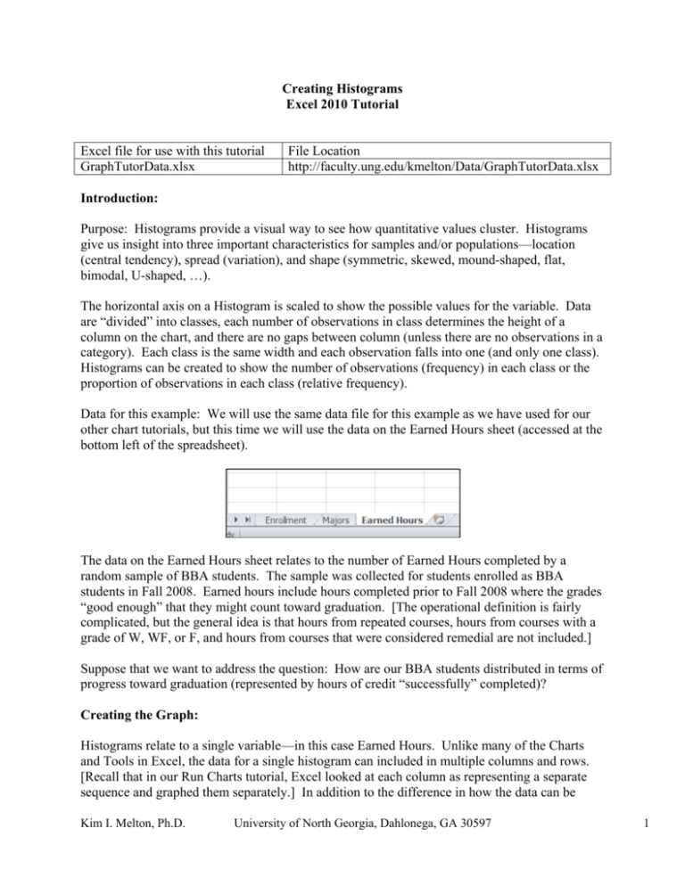
Creating Histograms
Excel 2010 Tutorial
Excel file for use with this tutorial
GraphTutorData.xlsx
File Location
http://faculty.ung.edu/kmelton/Data/GraphTutorData.xlsx
Introduction:
Purpose: Histograms provide a visual way to see how quantitative values cluster. Histograms
give us insight into three important characteristics for samples and/or populations—location
(central tendency), spread (variation), and shape (symmetric, skewed, mound-shaped, flat,
bimodal, U-shaped, …).
The horizontal axis on a Histogram is scaled to show the possible values for the variable. Data
are “divided” into classes, each number of observations in class determines the height of a
column on the chart, and there are no gaps between column (unless there are no observations in a
category). Each class is the same width and each observation falls into one (and only one class).
Histograms can be created to show the number of observations (frequency) in each class or the
proportion of observations in each class (relative frequency).
Data for this example: We will use the same data file for this example as we have used for our
other chart tutorials, but this time we will use the data on the Earned Hours sheet (accessed at the
bottom left of the spreadsheet).
The data on the Earned Hours sheet relates to the number of Earned Hours completed by a
random sample of BBA students. The sample was collected for students enrolled as BBA
students in Fall 2008. Earned hours include hours completed prior to Fall 2008 where the grades
“good enough” that they might count toward graduation. [The operational definition is fairly
complicated, but the general idea is that hours from repeated courses, hours from courses with a
grade of W, WF, or F, and hours from courses that were considered remedial are not included.]
Suppose that we want to address the question: How are our BBA students distributed in terms of
progress toward graduation (represented by hours of credit “successfully” completed)?
Creating the Graph:
Histograms relate to a single variable—in this case Earned Hours. Unlike many of the Charts
and Tools in Excel, the data for a single histogram can included in multiple columns and rows.
[Recall that in our Run Charts tutorial, Excel looked at each column as representing a separate
sequence and graphed them separately.] In addition to the difference in how the data can be
Kim I. Melton, Ph.D.
University of North Georgia, Dahlonega, GA 30597
1
entered, we will not be using the charts on the Insert tab to create this graph. Instead, we will use
the Histogram Tool in the Data Analysis Tools.
We will look at three ways to create a Histogram:
 Letting Excel do most of the work (including selecting the number and width of the classes)
[Sounds good, but definitely, not the recommended approach.]
 Determining the number of classes and the class widths based on the context of the situation
 Determining the number of classes and the class widths when the situation does not suggest
logical groupings.
Letting Excel do the work:
Step 1: Make sure that you have the Data Analysis Tools visible on the Data tab. If not add
them.
Step 2: From the Data tab at the top of the page, select Data Analysis and then select the
Histogram option.
To fill in the dialogue box, we need to understand some of the language that Excel uses. Input
Range refers to the location of the data that will be used to create the graph. [Excel will give
ignore blank cells and will give an error message if there are non-numeric values in any selected
cell.] Bin Range refers to the intervals used for each class. Excel uses the largest number in a
class to describe the class. If you do not provide input in this area, Excel will provide the
intervals (and it will ALWAYS provide a poor choice)! The Output options are similar to those
in other tools. And, although you might think that selecting the Histogram tool would tell Excel
to plot a histogram, you must check the box next to Chart Output if you what the graph.
To fill in the dialogue box for this example, click in the white box to the right of Input Range and
drag over the data (without any titles) to be used in the chart (in this case A2 through J26), leave
the Bin Range empty and do not click the labels box. To put your chart on the same page with
your data, click the button to the left of Output Range and click to white box to the right of
Output Range. Enter the cell that will be the upper left corner for your output—this example
used O1. Finally, click the box next to Chart Output. The completed dialogue box is shown
below:
Kim I. Melton, Ph.D.
University of North Georgia, Dahlonega, GA 30597
2
When you click Ok, you will see the following output:
Excel created six classes (bins) and a histogram that looks almost symmetric. When you do not
select the Bin Range, Excel will determine the number of classes, and will always include a
“More” class that has at least one observation in the interval! Also, Excel always shows space
between the classes/bins/columns.
Using our example to describe what is included in the output: The bin listed as 0 contains all
observations that are less than or equal to 0. In our example, we cannot have any students who
have completed less than 0 hours, so the 17 observations in this class represent students with no
completed hours posted to their transcripts (mostly new freshmen but could include transfer
students with transcripts that have not been entered and a few other situations). The bin listed as
36.8 includes all students with more than 0 earned hours up to and including students with 36.8
earned hours. Since students who have completed less than 30 hours are considered Freshmen,
we are left with no way to tell how many of these 50 students are Freshmen and how many are
Sophomores. The bin listed as 73.6 includes students who have earned credit for more than 36.8
hour and less than or equal to 73.6 hours. Some of these students would be Sophomores and
some would be Juniors. Following the same approach, the bin listed as 110.4 would include
some Juniors and some Seniors. All of the students in the bin listed as 147.2 would be classified
as Seniors. Finally, there are 5 students who have earned more than 147.2 hours—but we don’t
know how many more hours! [Note: Since the maximum value in the data set can be
determined, a “More” category should not be needed.]
Although there are multiple ways to determine the number of bins and the width of bins for a
histogram, some methods are better than others. Typically, larger data sets lead to using more
bins; the bins should be set up to include all observations in exactly one bin; and bins should be
selected in such a way that the “shape” of the distribution is not distorted. Obviously, Excel
needs some help to make better histograms!
Using class intervals based on the scenario:
Step 1: Identify how the classes/bins will be set up. Since our data represents progress toward
graduation, we could establish bins that align with the language we use in the university. We
generally refer to students who have completed less than 15 hours as first semester Freshmen, 15
hours to less than 30 hours as second semester Freshmen, 30 hours to less than 45 as first
semester Sophomores, and so on. Unfortunately, our language is slightly different from the way
that Excel “talks.” Mathematically, we would be saying that students with 15 ≤ Hours < 30
hours are second semester Freshmen; but Excel wants the intervals written with the < on the low
end and ≤ on the upper end. If we are willing to say that students who finished their 30th hour
Kim I. Melton, Ph.D.
University of North Georgia, Dahlonega, GA 30597
3
prior to this semester were still Freshmen in the previous semester, we can use 15, 30, 45, 60, 75,
… as the upper ends for our bins and tie this to student’s classification in a way that is easy to
communicate.
Step 2: Set up the bins in Excel. Since we have already selected the method to set bins, we
know that the upper limit of the first few will be 15, 30, and 45. We need to know the
maximum value in the data set in order to know how many bins to create (or how high to go).
Using =max(A2:J26), we find that the largest number in the data set is 184. Note, we will not
lump all observations above 120 hours into a single class since this would violate the need for all
classes to be the same width.
To tell Excel the class ranges, we create a column (labeled bins in the following diagram) that
lists the highest number in each class. We can take a short-cut by typing in the first two
endpoints to set the pattern. In this illustration, we typed the heading in A32 and the first two
entries in A33 and A34. Then highlight these two entries and move the cursor to the lower right
corner of the highlighted cells until it turns to a black plus sign.
Drag down the column until you reach the first value that it higher than 184 (the maximum value
in the data set).
Step 3: Use the Histogram Tool in the Data Analysis Tools to obtain the initial chart.
To complete the Histogram dialogue box, drag over all of the data to provide the input range.
Then drag over the numbers you created for the upper endpoint for each bin to provide the
information Excel needs for the Bin Range (do not select the heading). If you want to put your
output on the same sheet that you have been working on, click next to Output Range, click in the
white box to the right of there, and give Excel information about the upper left cell to contain the
output—I selected the cell to the right of where I typed the word “Bins.” Finally, click next to
Chart Output.
Kim I. Melton, Ph.D.
University of North Georgia, Dahlonega, GA 30597
4
Click OK to obtain the following graph.
Step 4: Clean up the Chart (delete the “Frequency” legend, get rid gap between the columns, and
get rid of the “More” class)
To remove the “Frequency” legend, click on it and hit the delete key.
To get rid of the extra space between the bars, right click on the one of the bars and select
Format Data Series from the resulting menu.
Move the indicator for the Gap Width to No Gap and click OK.
Kim I. Melton, Ph.D.
University of North Georgia, Dahlonega, GA 30597
5
To get rid of the “More” class, click on one of the blue bars and notice that the data used to
create the graph is highlighted. Carefully, move the lower end of the boxes highlighting the data
so that the last row is not selected.
Step 5: Add/revise the axis label and a Chart Title
Setting up class intervals when the scenario doesn’t provide guidance: Although we did have a
logical way to set up our bins for the earned hours, we will use the same data to illustrate how we
would proceed if we had not recognized this.
Step 1: Determine the number of classes/bins to use. When there is no obvious (or generally
accepted way of grouping the data), we use the number of observations in the data set to help
determine the appropriate number of bins to construct. We want enough bins to see the spread in
the observations; but few enough bins to see the clustering of observations. As a general rule,
the more data, the more bins. One easy to remember approach that generally works fine when
you have less than 100 observations is to take the square root of the number of observations as a
suggestion for the number of bins. [For example, if you had 75 observations you would want
approximately 8 or 9 bins. Could you use 7 or 10? Yes. Could you use 2 or 15? Probably not
the best choices!] With larger data sets, you will need to use more judgment about adding more
bins.
In our example, we have 250 observations where the numbers range from 0 to 184. We would
like to create bins that cover this entire range with very little “extra” room. If we were to set up
Kim I. Melton, Ph.D.
University of North Georgia, Dahlonega, GA 30597
6
16 bins, each bin would need to be (184 -0)/16 =11.5 units wide [where 184 – 0 gives the total
width that needs to be covered].
Step 2: Set up the bins in Excel
Using the same approach as in the previous chart, we type in the first two upper endpoints for the
bins (11.5 and 23) to set the pattern; then we highlight these two entries, move the cursor to the
lower right of the highlighted cells until it becomes a black plus sign and drag down the column
until we reach 184.
Once these steps are complete, follow the same steps that we did when the scenario helped
dictate the bins. The initial output from Excel and the final histogram are shown below.
Communicating the Results:
Communicating results: From the histogram created using the 15 hour blocks, we can see that
the distribution is fairly flat up to about 75 semester hours completed, then is a little higher from
there to 120 completed hours, but drops off considerably after that. Since these data were
obtained when a large number of students transferred into the BBA program (from other schools
or by changing their majors), the increase toward the end of the sophomore year is logical. Also,
since students are required to complete 120 semester hours to graduate, the drop off after 120 is
reasonable. We could say the distribution is right skewed (or positively skewed) based on the
Kim I. Melton, Ph.D.
University of North Georgia, Dahlonega, GA 30597
7
classes on the right with low counts. In addition, we might question if the two highest
observations – that are set apart from the rest of the observations – were outliers (potentially the
data were recorded incorrectly or the students were mis-classified as undergraduates).
Caution: There is an assumption that all of the data are drawn from a single homogeneous
population. When this is the case, we do not need to worry about the fact that histograms ignore
the time order of the data. But when there are systematic changes occurring while data are being
collected, histograms can be misleading (as insight into location, spread and shape). For
example, consider the following two situations. For each situation, you are provided a Run Chart
and a Histogram created from the data displayed on the Run Chart. Even though the Run Charts
look very different, the Histograms are identical. The Run Charts show the data in the sequence
that the observations were produced; but the Histograms ignore the order that the data were
created. In this example, the only difference between the two data sets is the order of the
observations!
Checklist:
 Determine the bins for the chart (the number, width, and upper endpoint for each interval)
 Select the Data Analysis Tools from the Data tab and use the Histogram tool
 Clean up any chartjunk (Frequency legend, space between columns, “More” category)
 Add/revise axis titles
 Add a title on the chart
 Position your chart on the page so that it will print on a single page (without page breaks
in the middle of the chart).
Kim I. Melton, Ph.D.
University of North Georgia, Dahlonega, GA 30597
8