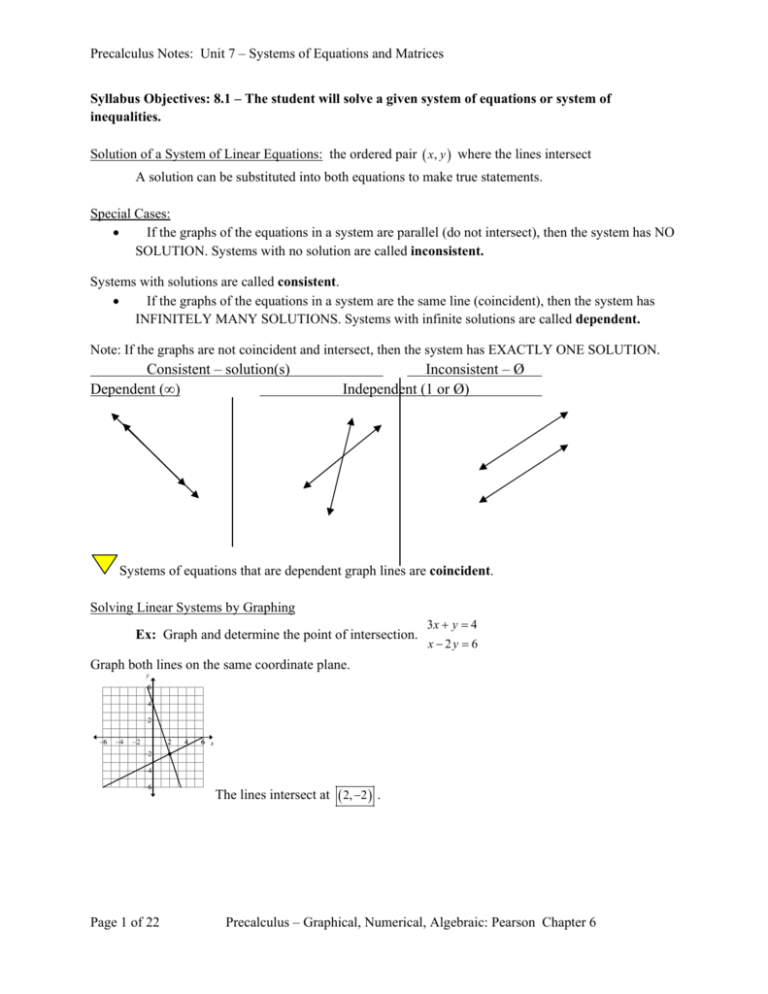
Precalculus Notes: Unit 7 – Systems of Equations and Matrices
Syllabus Objectives: 8.1 – The student will solve a given system of equations or system of
inequalities.
Solution of a System of Linear Equations: the ordered pair  x, y  where the lines intersect
A solution can be substituted into both equations to make true statements.
Special Cases:

If the graphs of the equations in a system are parallel (do not intersect), then the system has NO
SOLUTION. Systems with no solution are called inconsistent.
Systems with solutions are called consistent.

If the graphs of the equations in a system are the same line (coincident), then the system has
INFINITELY MANY SOLUTIONS. Systems with infinite solutions are called dependent.
Note: If the graphs are not coincident and intersect, then the system has EXACTLY ONE SOLUTION.
Consistent – solution(s)
Dependent (∞)
Inconsistent – Ø
Independent (1 or Ø)
Systems of equations that are dependent graph lines are coincident.
Solving Linear Systems by Graphing
Ex: Graph and determine the point of intersection.
3x  y  4
x 2y  6
Graph both lines on the same coordinate plane.
y
x
The lines intersect at  2, 2  .
Page 1 of 22
Precalculus – Graphical, Numerical, Algebraic: Pearson Chapter 6
Precalculus Notes: Unit 7 – Systems of Equations and Matrices
Solving a System by Graphing (not linear)
Ex: Graph and find the solution of the system.
3x  2 y  6
y  ln  x  1
Graph both functions on the same coordinate plane.
y
x
The solution of the system is the point at which the functions intersect:  2,0 
Solving a System of Linear Equations by Substitution
Ex: Solve using substitution.
3 x  y  7
6 x  2 y  8
Step One: Solve one of the equations for one of
the variables (if necessary). Note: You may
choose which variable to solve for.
Step Two: Substitute the expression from Step
One into the other equation of the system and
solve for the other variable.
Note: Both variables were eliminated, and the
resulting equation is an untrue statement. If the
resulting equation was a true statement, then the
lines are coincident and there are infinitely many
solutions.
Page 2 of 22
3 x  y  7
y  3x  7
6 x  2  3 x  7   8
6 x  6 x  14  8
14  8
No Solution (The lines are parallel.)
Precalculus – Graphical, Numerical, Algebraic: Pearson Chapter 6
Precalculus Notes: Unit 7 – Systems of Equations and Matrices
Solving Nonlinear Systems by Substitution
Ex: Solve the system.
x 2  y 2  13
y  x2  1
Step One: Solve one of the equations for one of
the variables (if necessary).
Step Two: Substitute the expression from Step
One into the other equation of the system and
solve for the other variable.
Step Three: Substitute the value from Step Two
into the equation from Step One and solve for
the remaining variable.
y  x2  1
x2  y  1
x 2  y 2  13
 y  1  y 2  13
y 2  y  12  0
x2  y  1
2
x  4  1
2
x  3
 y  4  y  3  0
y  4, 3
x2  3  1
x2  4
x  2
No Solution
Step Four: Write your answer as an ordered pair
and check in both of the original equations.
Solutions:
 2,3 ,  2,3
Note: We solved for x 2 instead of substituting the expression for y to avoid a high-degree
polynomial equation to solve.
Page 3 of 22
Precalculus – Graphical, Numerical, Algebraic: Pearson Chapter 6
Precalculus Notes: Unit 7 – Systems of Equations and Matrices
Solving Linear Systems by Linear Combinations (Elimination)
Ex: Solve the system.
3 y  5 x  1
4 x  6 y  10
Step One: Write the two equations in standard
form.
5x  3 y  1
Step Two: Multiply one or both of the equations
by a constant to obtain coefficients that are
opposites for one of the variables.
5 x  3 y  1  10 x  6 y  2
4 x  6 y  10
4 x  6 y  10  4 x  6 y  10
6 x  0 y  12
Step Three: Add the two equations from Step
Two. One of the variable terms should be
eliminated. Solve for the remaining variable.
6 x  12
x2
5  2  3 y  1
Step Four: Substitute the value from Step Three
into either one of the original equations to solve
for the other variable.
10  3 y  1
 3 y  9
y3
Step Five: Write your answer as an ordered pair
and check in the original system.
Solution:
 2,3
Application Problems – Systems of Equations
Ex: Three gallons of a mixture is 60% water by volume. Determine the number of gallons of
water that must be added to bring the mixture to 75% water.
Assign labels: w = gallons of water; t = total gallons of mixture
3 w  t
Write a system:
Amount (gallons)
Value (percent water) 3  0.60   w 1.00   t  0.75
Solve the system:
Rewrite second equation.
Use substitution.
Page 4 of 22
1.8  w  .75t  180  100 w  75t
180  100 w  75  3  w 
180  100 w  225  75w
25w  45
w  1.8 gallons
Precalculus – Graphical, Numerical, Algebraic: Pearson Chapter 6
Precalculus Notes: Unit 7 – Systems of Equations and Matrices
Ex: A machine takes 3 minutes to form a bowl and 2 minutes to form a plate. The material costs
$0.25 for a bowl and $0.20 for a plate. How many bowls and plates were made if the machine
ran for 8 hours and $44 was spent on materials?
Assign labels: b = # of bowls; p = # of plates
3b  2 p  8  60  Multiply by 60 to change hours to minutes.
Write a system:
Time
Money
Solve the system:
0.25b  0.20 p  44
Rewrite equations.
30b  20 p  4800
Use elimination.
25b  20 p  4400
5b  400
b  80
3b  2 p  480
25b  20 p  4400
3 80   2 p  480
2 p  240
p  120
Solution:
80 bowls, 120 plates
You Try:
x  y  6

x y
2
 x  y   6  x
1. Solve the system: 
(Hint: You do not need to substitute for a single variable. You can use an expression.)
2. A car radiator contains 10 quarts of a 30% antifreeze solution. How many quarts will have to be
replaced with pure antifreeze if the resulting solution is to be 50% antifreeze?
QOD: Explain how you would choose the most efficient method for solving a system of equations.
Page 5 of 22
Precalculus – Graphical, Numerical, Algebraic: Pearson Chapter 6
Precalculus Notes: Unit 7 – Systems of Equations and Matrices
Syllabus Objectives: 8.2 – The student will calculate the determinant of a square matrix. 8.3 – The
student will find the inverse of a given square matrix.
Matrix: a rectangular arrangement of numbers (called entries) in rows and columns.
Plural of matrix: matrices
Dimensions (Order) of a Matrix: Number of Rows  (“by”) Number of Columns
1 1

5
A= 0


 3 2 
Entry/Element
a32 = −2 (row 3, column 2)
Matrix A is a 3x2 matrix.
Square Matrix: a matrix with the same number of rows and columns
Ex: Determine the order of the matrix. Is it a square matrix? Identify b24 .
2 5 1 4
B4 8 0 6


 3 1 2 1
Order: Rows by Columns
3 4
No, it is not a square matrix.
b24 : Element in row 2, column 4 b24  6
Adding and Subtracting Matrices: matrices must have the same order
Add or subtract corresponding elements.
Multiplying by a Scalar: multiply all elements of the matrix by the scalar
2
0
 4 8 
2 
Ex: Perform the operations. 
  2 0
 7 1

Multiply by the scalar:
 2 0   8 16 
 7 1   0 4 

 

Add the matrices:
0  16   6 16 
 2   8 


1   4   7 5
 70
Matrix Multiplication: In order to multiply matrices, the number of columns in the first matrix must equal
the number of rows in the second matrix. The product matrix will have the same number of rows of the
first matrix and the same number of columns of the second matrix.
Matrix multiplication is NOT commutative. ( AB  BA for all matrices A and B.)
Page 6 of 22
Precalculus – Graphical, Numerical, Algebraic: Pearson Chapter 6
Precalculus Notes: Unit 7 – Systems of Equations and Matrices
Let A be an m  n matrix, and B be an n  p matrix. The product A  B exists, and will have the
dimensions m  p .
2 3
 4 1
Ex: Find the product AB (if possible). A   1 5  B  


3 6

 0 2 
Step One: Determine if the product exists. If it does, find its dimensions.
Matrix A is a 3  2 matrix. Matrix B is a 2  2 matrix. The number of columns in
matrix A equals the number of rows in matrix B. Therefore, the product exists and will be
a 3  2 matrix.
Step Two: Multiply each entry in the rows of matrix A to each entry in the columns of matrix B.
Then find the sum of these products.
2 1  3  6  
 2  4   3  3


 1 4   5  3 1 1  5  6   
 0  4   2  3 0 1  2  6  
 1 20 
 19 29 


 6 12 
Ex: Find the product BA (if possible) of the matrices from the previous example.
Step One: Determine if the product exists. If it does, find its dimensions.
Matrix B is a 2  2 matrix. Matrix A is a 3  2 matrix. The number of columns in Matrix
B does not equal the number of rows in matrix A. Therefore, the product BA does not
exist.
Matrices on the Graphing Calculator
Ex: Evaluate the product from the previous example on the graphing calculator.
In the Matrix Menu, choose Edit, then Matrix A. Our matrix is a 3  2 , so enter in the dimensions. Then
enter in the entries of the matrix. Keystrokes:
Enter Matrix B the same way.
Page 7 of 22
On the home screen, you can perform matrix operations.
Precalculus – Graphical, Numerical, Algebraic: Pearson Chapter 6
Precalculus Notes: Unit 7 – Systems of Equations and Matrices
Recall:
Identity of Addition: a  0  a
Identity of Multiplication: a  1  a
1 0
 0 0
Matrix Identity of Multiplication: 

0 1
Matrix Identity of Addition: 

 0 0
 1 2   1 0 
 1 2   0 0 
and 


.
4  0 0
 3 4  0 1
Ex: Find 
3
 1 2   0 0  1 2 
 3 4    0 0   3 4 

 
 

 1 2  1 0  1 2 
 3 4   0 1   3 4 

 
 

Recall:
Additive Inverse: a   a   0
Multiplicative Inverse: a 
b   a
a
b 
1
1
a
0 0
Additive Inverse (matrices): 



 c d   c d  0 0
a b 
 , then det  A  A  ad  bc .
c d 
Determinant of a Matrix: If A  
Nonsingular Matrix: a matrix that has a nonzero determinant
a
b
1 d
1
Inverse of a 2×2 Matrix: If A  
 , then A  A   c
c d 

b 
, A  0.
a 
1 0
 , the multiplicative identity.
0 1
The product of A  A1  A1  A  
Note: If A  0 , then A does not have an inverse. Be careful with notation. A1 means the inverse
of matrix A, NOT the reciprocal of matrix A.
 4
Ex: Find the inverse of B  
6
1
. Verify your answer.
2 
Evaluate the determinant:
B  4  2   1  6   2
Write the inverse:
B 1 
1

1  2 1
1
 1  2 
B




2  6 4 
 3 2 
Verify by multiplying:


 1
4     1  2  
1   4  1  1  3


4
1
1 0


1
2




  

B  B 1  
2  

☺
 6 2   3 2   6 1  2 3 6   1   2 2  0 1 

      

   
 2


Page 8 of 22
Precalculus – Graphical, Numerical, Algebraic: Pearson Chapter 6
Precalculus Notes: Unit 7 – Systems of Equations and Matrices
Evaluating the Determinant of a 3×3 Matrix: Lattice Method
Ex: Evaluate the determinant.
4 2 3
5 1 0
2 1 11
rd
Rewrite the first two columns to the right of the 3 column:
4 2 3 4 2
5 1 0 5 1
2 1 11 2 1
Multiply along the diagonals. Find the sum of the products of the diagonals from left to right and the
opposite of the products of the diagonals from right to left. (Blue – Red)
4
2 3
4
2
5 1 0 5 1
2 1 11 2 1
4 2 3
5 1 0  87
2 1 11
−(6 + 0 + 110) + (44 + 0 + −15)
−116 + 29 = −87
Evaluating an Inverse on the Graphing Calculator
Ex: Calculate the determinant of the matrix on the calculator. Then find the inverse and verify.
 0 2 1
A   1 1 1 


 2 3 0 
Enter the matrix into the calculator.
On the home screen, find the determinant.
det( can be found in the Matrix Math menu.
Find the inverse:
Verify:
 2 6 
You Try: Find the A1 . Then verify that it is the inverse of A. A  
.
 1 5
QOD: Which matrix operation(s) are commutative? Explain.
Page 9 of 22
Precalculus – Graphical, Numerical, Algebraic: Pearson Chapter 6
Precalculus Notes: Unit 7 – Systems of Equations and Matrices
Syllabus Objective: 8.4 – The student will solve application problems involving matrix operations
with and without technology.
Triangular Form of a System: an equivalent form of a system from which the solution is easy to read; all
lead coefficients are equal to 1
x  2 y  2z  7
Ex: Solve the system in triangular form.
y  2 z  7
z3
Use back substitution:
y  2  3   7  y  1
x  2  1  2  3  7  x  11
Write solution as an ordered triple: 11, 1,3
Gaussian Elimination: transforming a system to triangular form by
 interchanging any two equations of the system
 multiplying (or dividing) one of the equations by any nonzero real number
 adding a multiple of one equation to any other equation in the system
2x  y  z  0
Eq. I
Ex: Solve the system using Gaussian Elimination. x  y  2 z  3 Eq. II
 x  2 y  3z  7 Eq. III
x  y  2 z  3
Switch Eq. I & Eq. II (leading coefficient of 1 on x-term): 2 x  y  z  0
Eq. I
Eq. II
 x  2 y  3z  7 Eq. III
x  y  2 z  3
 x  2 y  3z  7
Add Eq. I + Eq. III:
x  y  2 z  3
We now have: 2 x  y  z  0
3 y  5z  6
Eq. III
x  y  2 z  3
We now have:
3 y  5z  6
yz4
Eq. I
Eq. II
Eq. III
x  y  2 z  3
Switch Eq. II & Eq. III (leading coefficient of 1 on y-term):
yz4
3 y  5z  6
3 y  3z  12
Add −3(Eq. II) + Eq. III:
Eq. II
yz4
yz4
2 x  2 y  4 z  6
Add −2(Eq. I) + Eq. II: 2 x  y  z  0
Eq. I
3 y  5z  6
 2 z  6  z  3
Eq. I
Eq. II
Eq. III
x  y  2 z  3
yz4
Triangular Form:
z3
Now that we have the system in the triangular form, solve by back substitution. Solution:  2, 7, 3
Page 10 of 22
Precalculus – Graphical, Numerical, Algebraic: Pearson Chapter 6
Precalculus Notes: Unit 7 – Systems of Equations and Matrices
Special Systems: A linear system can have exactly one solution, infinitely many solutions, or no solution.
x  2y  z  4
Ex: Solve the system. 3x  6 y  3z  7
2x  y  4z  2
3x  6 y  3z  12
3 x  6 y  3z  7
Add −3(Eq. I) + Eq. II:
0  5
All variables were eliminated, and the result is a false statement. Therefore, this system has NO
SOLUTION (the lines do not intersect).
a1 x  b1 y  c1 z  d1
Coefficient Matrix of a System: The coefficient matrix of the system a2 x  b2 y  c2 z  d 2
a3 x  b3 y  c3 z  d 3
is
 a1
a
 2
 a3
b1
b2
b3
c1 
c2  .

c3 
a1 x  b1 y  c1 z  d1
Augmented Matrix of a System: The augmented matrix of the system
a2 x  b2 y  c2 z  d 2
a3 x  b3 y  c3 z  d 3
is
 a1
a
 2
 a3
b1
c1
b2
b3
c2
c3
d1 
d2  .

d 3 
Row Echelon Form of a Matrix: the augmented matrix that corresponds to the triangular form of the
original system of equations
 rows consisting entirely of zeros (if any) occur at the bottom of the matrix
 the first entry in any row with nonzero entries is 1
 the column subscript of the leading 1 entries increases as the row subscript increases (the
leading 1’s move to the right as we move down the rows)
1 1 2 3
y  z  4 as an augmented matrix:  0 1 1 4 


 0 0 1 3 
z3
x  y  2 z  3
For Example, the triangular system
We will write a system as an augmented matrix, then use Elementary Row Operations to put the matrix
in Row Echelon Form to solve the system. Elementary Row Operations:
 interchange rows
 multiply all elements of a row by a nonzero number
 add a multiple of one row to any other row
Page 11 of 22
Precalculus – Graphical, Numerical, Algebraic: Pearson Chapter 6
Precalculus Notes: Unit 7 – Systems of Equations and Matrices
Note: These are the same strategies we used in Gaussian Elimination! Tip: Start in the lower left
corner of the matrix.
3x  2 y  z  5
Ex: Solve the system using an augmented matrix in row echelon form. x  y  z  4
x  3 y  2 z  3
3
2
1
3
Write as an augmented matrix: 1 1
1 5
1 4

2 3
3 2 1 5 
 1 1 1 4 


Perform the elementary row operations: 1 1 1 4   R1  R 2  3 2 1 5   3R1  R 2 
1 3 2 3
1 3 2 3
4
4
4
1 1 1
 1 1 1
 1 1 1 4 
 1 1 1
 0 5 2 7    R1  R 3   0 5 2 7    R 3  R 2  0 1 1 0   4 R 2  R3  0 1 1
0








1 3 2 3
 0 4 3 7 
0 4 3 7 
0 0 7 7 
1 1 1 4 
1
  R 3   0 1 1 0  Row Echelon Form!


7
 0 0 1 1 
Triangular Form of System:
x yz 4
yz0
z 1
Solution of System (use back substitution):  2, 1,1
Reduced Row Echelon Form: every column that has a leading 1 has zeros elsewhere
Ex: Write the augmented matrix above in reduced row echelon form.
1 1 1 4 
1 1 1 4 
 1 1 0 3 
1 0 0 2 
 0 1 1 0    R 3  R 2   0 1 0 1   R 3  R1  0 1 0 1  R 2  R1  0 1 0 1








 0 0 1 1 
 0 0 1 1 
0 0 1 1 
0 0 1 1 
1 0 0
2
 0 0 1
1 
Reduced Row Echelon Form: 0 1 0 1
Solution of system is the last column!  2, 1,1
Special Case: Infinite Solutions
x  y  3  1
Ex: Solve the system.
yz0
x  2 y
1
 1 1 3 1
1 1 3 1
1 1 3 1
1 1 3 1
 0 1 1 0   R1  R 3  0 1 1 0   1 R 3  0 1 1 0    R 2  R 3  0 1 1 0 



 3




 1 2 0 1 
0 3 3 0 
0 1 1 0 
0 0 0 0 
Notice that the last row in the matrix represents the equation 0 = 0, so we know there are infinitely many
solutions. We can represent these solutions as an ordered triple in terms of z.
yz 0  y  z
x  y  3 z  1  x   y  3 z  1  x   z  3 z  1  x  2 z  1
Page 12 of 22
Solutions:  2 z  1, z, z 
Precalculus – Graphical, Numerical, Algebraic: Pearson Chapter 6
Precalculus Notes: Unit 7 – Systems of Equations and Matrices
1
a
Recall: Inverses can be used to solve the equation a  x  b . x   b
Solving Systems Using Inverses: The system
a
 x
b
1
a1 x  b1 y  c1
a
b   x
c 
can be written as  1 1       1  . So the
a2 x  b2 y  c2
 a2 b2   y   c2 
c 
solution of the system is     1 1    1  .
 y   a2 b2   c2 
a
b
Note: The matrix  1 1  is called the coefficient matrix.
 a2 b2 
Ex: Solve the system
4 x  y  4
6x  2 y  3
 4
Write as a matrix equation: 
6
using the inverse matrix.
1   x  4

2   y   3
 4 1 
Find the inverse of the coefficient matrix: 

 6 2 
Multiply both sides by the inverse:
1

 2 1 1  2 1
1

 4  2   1 6   6 4  2  6 4 
1  2 1  4 1   x  1  2 1  4 



2  6 4   6 2   y  2  6 4   3
Note: Multiplying the coefficient matrix by its inverse results in the identity matrix.
 11 
 x  1  2 1  4  1  2  4    1 3  1  11   
2
 
  
   

 y  2  6 4   3 2  6  4    4  3  2  36  18 


11
Solution:   , 18 

2

Solving a System Using Inverse Matrices
x  y z w4
Ex: Solve the system.
2x  y
z
0
3x  2 y  z  w  6
x  2 y  2 z  2 w  1
Write as a matrix equation:
1 1 1 1   x   4 
 2 1 1 0   y   0 

    
 3 2 1 1  z   6 

   
 1 2 2 2   w   1
Enter the coefficient matrix as Matrix A and the constant matrix as Matrix B.
Multiply A1  B .
Page 13 of 22
Solution: 1, 2,0,1
Precalculus – Graphical, Numerical, Algebraic: Pearson Chapter 6
Precalculus Notes: Unit 7 – Systems of Equations and Matrices
Application Problems
Ex: A man borrows a total of $10,000; some at 18%, 15%, and 9%. He borrows 3 times as much
at 15% as he borrows at 18%, and the total interest on all of the loans is $1244.25. How much
did he borrow at each percentage rate?
Assign labels: x = amount borrowed at 18%; y = amount at 15%; z = amount at 9%
x  y  z  10000
Write a system:
Total amount borrowed:
Total interest:
0.18 x  0.15 y  0.09 z  1244.25
Other information given:
3x  y   3x  y  0
1
Solve by inverses:
1
1   x   10000 
1
1   10000 
 1
x  1
0.18 0.15 0.09   y   1244.25   y   0.18 0.15 0.09   1244.25

  

  
 

1
0   z   0 
1
0   0 
 3
 z   3
He borrowed $1275 at 18%, $3825 at 15%, and $4900 at 9%.
Ex: Determine the quadratic function that contains the points 1, 3 ,  2,10  , &  2, 6  .
Quadratic function: y  ax 2  bx  c
We must find a, b, and c.
2
Substitute each ordered pair into y  ax  bx  c .
1 1 1  a   3 
 4 2 1  b   10 

   
 4 2 1  c   6 
a   1 
b    4 
   
 c   2 
 a  1 1 1
 b    4 2 1
  

 c   4 2 1
1
3  abc
1,3 :
 2,10  : 10  4a  2b  c
 2, 6  :  6  4a  2b  c
3
10  Solve on graphing calculator.
 
 6 
Solution: y  x 2  4 x  2
You Try: 1. Solve the system from the second application problem using reduced row echelon form.
2. A piggy bank contains quarters, dimes, and nickels. The number of dimes is 1 less than the number of
nickels. The number of nickels is 2 more than twice the number of quarters. The coins are worth $5.70.
How many nickels are there?
QOD: When solving systems using inverse matrices, does it matter which order you multiply by the
inverse matrix? Explain.
Page 14 of 22
Precalculus – Graphical, Numerical, Algebraic: Pearson Chapter 6
Precalculus Notes: Unit 7 – Systems of Equations and Matrices
Syllabus Objective: 8.5 – The student will use partial fractions to decompose rational expressions
with distinct linear factors.
Recall: To add the rational expressions
3
2
, we must find a common denominator.

x4 x3
3  x  3  2  x  4  3x  9  2 x  8
3
2
5x  1



 2
x4 x3
 x  4  x  3 x  x  12
 x  4  x  3
What if we wanted to go from the sum,
or
a c ad  bc
 
b d
bd
5x  1
3
2
, back to the addends,
?

x4 x3
x  x  12
2
Partial Fraction Decomposition: writing rational expressions as the sum of simpler ones
Steps – Case I: Distinct (no repeated) Linear Factors in the Denominator
1. Factor the denominator.
2. Write the factors as a sum.
3. Clear the fractions (multiply by the LCD).
4. Write and solve the resulting system of equations.
5. Write the resulting partial fractions.
5 x  10
.
2 x 2  3x  2
5 x  10
5 x  10

2
2 x  3x  2  2 x  1 x  2 
Ex: Find the partial fraction decomposition of
1. Factor the denominator:
2. Write the factors as a sum.
5 x  10
A
B


 2 x  1 x  2   2 x  1  x  2 
5 x  10  A  x  2   B  2 x  1
3. Clear the fractions.
5 x  10  Ax  2 A  2 Bx  B
4. Write and solve the system.
5 x  10  Ax  2 Bx  B  2 A
   2    2 A  4 B  10
A  2B  5
2 A  B  10

2 A  B  10
 5B  20  B  4
5. Write the resulting partial fractions.
Solution:
Page 15 of 22
A  2B  5
5 x  10   A  2 B  x   2 A  B 
2 A  B  10
A  2B  5
A  2 4  5
A  3
5 x  10
A
B
3
4




 2 x  1 x  2   2 x  1  x  2   2 x  1  x  2 
4
3

x  2 2x 1
Precalculus – Graphical, Numerical, Algebraic: Pearson Chapter 6
Precalculus Notes: Unit 7 – Systems of Equations and Matrices
Steps – Case II: Repeated Linear Factors in the Denominator
1. Factor the denominator.
2. Write the factors as a sum. Any repeated factors, f n will be written as n factors in the fractions.
A
A A1 A2

 2  ...  nn
n
f
f
f
f
3. Clear the fractions (multiply by the LCD).
4. Write and solve the resulting system of equations.
5. Write the resulting partial fractions.
x2
as a decomposition of partial fractions.
x  2x 1
x2
x2
1. Factor the denominator.

2
x  2 x  1  x  12
Ex: Write
2
2. Write the factors as a sum. Any repeated factors, f n will be written as n factors in the fractions.
x2
 x  1
2

A
B

 x  1  x  12
x  2  A  x  1  B  x  2  Ax  A  B
3. Clear the fractions (multiply by the LCD).
4. Write and solve the resulting system of equations.
A 1
1  B  2
A B  2
B3
x2
1
3


x 2  2 x  1 x  1  x  12
5. Write the resulting partial fractions.
Steps – Case III: Irreducible Distinct Quadratic Factors in the Denominator
1. Factor the denominator.
2. Write the factors as a sum. Any irreducible quadratic factor in the denominator must have a
linear expression in the numerator, i.e.  ax  b  .
3. Clear the fractions (multiply by the LCD).
4. Write and solve the resulting system of equations.
5. Write the resulting partial fractions.
Ex: Find the partial fraction decomposition of
8 x 2  5 x  18
x
3
8
1. Factor the denominator (difference of two cubes).

.
8 x 2  5 x  18
x
3
8


8 x 2  5 x  18
 x  2  x2  2 x  4
2. Write the factors as a sum. Any irreducible quadratic factor in the denominator must have a
linear expression in the numerator, i.e.  ax  b  .
8 x 2  5 x  18
 x  2  x
2
 2x  4


A
Bx  C
 2
x

2

 x  2x  4


3. Clear the fractions (multiply by the LCD).
Page 16 of 22


8 x 2  5 x  18  A x 2  2 x  4   Bx  C  x  2 
2
2
8 x  5 x  18  Ax  2 Ax  4 A  Bx 2  2 Bx  Cx  2C
Precalculus – Graphical, Numerical, Algebraic: Pearson Chapter 6
Precalculus Notes: Unit 7 – Systems of Equations and Matrices
4. Write and solve the resulting system of equations.
8 x  5 x  18   A  B  x   2 A  2 B  C  x   4 A  2C 
A B
8
2 A  2B  C  5
4A
 2C  18
0 8
0 8
1 1
1 1
1
 2 2 1 5   2 R 2  R 3  2 2 1 5  2 R1  R 2 0





 4 0 2 18
 0 4 4 8
0
1 1 0 8 
1 1 0 8 
1 1
R3 
R2 



0 4 1 11  R 3  R 2 0 4 0 12
0 1


 4 
3 
0 0
0 0 1 1 
0 0 1 1 
1
0
8 
1

4 1 11 R 2  R3 0


4 4 8 
0
0 8
1 0 0

0 3  R 2  R1 0 1 0


1 1
0 0 1
2
2
5. Write the resulting partial fractions.
1 0
8 
4 1 11

0 3 3 
5
3 A  5, B  3, C  1

1
8 x 2  5 x  18
5
3x  1


x  2 x2  2x  4
x3  8
Irreducible Quadratic Factors
Ex: Find the partial fraction decomposition.
x3  x 2  5x  2
x
2
3

2

Ax  B
x
2
3

 x
3

x
2
3

2


x 3  x 2  5 x  2   Ax  B  x 2  3  Cx  D
Cx  D
2
x3  x2  5x  2
2
x 3  x 2  5 x  2  Ax 3  3 Ax  Bx 2  3B  Cx  D
A 1
x 3  x 2  5 x  2  Ax 3  Bx 2   3 A  C  x   3B  D 
x3  x 2  5x  2
x
2
3

2

B  1
3 1  C  5
3  1  D  2
3A  C  5
3B  D  2
C2
D 1
x 1
2x 1

2
x  3 x2  3 2


Improper Fractions: use long division to write in the form q  x  
Ex: Find the partial fraction decomposition.
r  x
d  x
4 x3  9 x 2  2 x  2
x  x  2
4 x  6
x2  2x
2
3
2
Long Division: x  2 x 4 x  9 x  2 x  2
Decompose:
4 x  6  A  x  2   Bx
A3
4x 1
4 x  6  Ax  2 A  Bx
4 x  6   A  B  x  2 A
A  B  4
2A  6
3  B  4
B  7
4 x  6 A
B
 
x  x  2 x x  2
4 x  6 3
7
 
x  x  2 x x  2
4 x3  9 x 2  2 x  2
3
7
 4x 1 
x  x  2
x x2
Page 17 of 22
Precalculus – Graphical, Numerical, Algebraic: Pearson Chapter 6
Precalculus Notes: Unit 7 – Systems of Equations and Matrices
You Try: Find the partial fraction decomposition of
3x 3  6 x 2  7 x  2
x
2
 2x  2

2
.
QOD: Are partial fraction decompositions always unique? Explain.
Page 18 of 22
Precalculus – Graphical, Numerical, Algebraic: Pearson Chapter 6
Precalculus Notes: Unit 7 – Systems of Equations and Matrices
Syllabus Objective: 2.1 – The student will graph relations or functions, including real-world
applications.
Half-Plane: the graph of a linear inequality
Number Line
Coordinate Plane
Open dot
Dotted (dashed) line
 & 
Closed (solid) dot
Solid Line
Note: You can use a test point to determine which half-plane to shade.
 & 
Ex: Draw the graph of the inequality. y  3x  4
Graph the line y  3x  4 , or y  3x  4 . The line will be “dashed” because it is a < sign.
y  3x  4
Pick a test point:  0,0 
0  0  4 true
Shade the half-plane that contains the test point.
y
x
Solution of a System of Inequalities: the intersection of the solutions of all of the inequalities in the
system; common solutions to all
x4
Ex: Graph and determine if the solution is bounded or unbounded. y  3
x y 4
y
x
To be sure we shaded the correct region, use a test point.
x4
Test Point  3, 2  : y  3
3 4
 2  3
☺
The region is bounded.
x  y  4 3   2   4
Page 19 of 22
Precalculus – Graphical, Numerical, Algebraic: Pearson Chapter 6
Precalculus Notes: Unit 7 – Systems of Equations and Matrices
Ex: Graph the system of inequalities and state if the solution is bounded or unbounded.
1 2
x 1
2
x 1
y
y
x
The region is unbounded.
Ex: Solve the system of inequalities.
y   x 1  3
x2  y2  9
y   x  1  3 : vertex at 1, 3 ; opens down; shade above
x 2  y 2  9 : circle with center  0,0  ; radius = 3; shade inside
Solution is the shaded region they have in common.
Linear Programming: decision making by finding a minimum or maximum value of a linear function
given a set of constraints
Constraints: a system of linear inequalities
Feasible Region: the solution set found using the constraints
Objective Function: an equation applied to a feasible region that we want to minimize or maximize
Vertex Points: the corner points of the feasible region
The maximum or minimum of a linear programming problem always occurs at a vertex point.
Solving a Linear Programming Problem
 Write the system of inequalities that represent the constraints.
 Graph the feasible region.
 Write the objective function.
 Test the vertex points in the objective function and answer the question.
Ex: Mrs. Arquette is baking as many cakes and pies as possible using the 18 eggs and 15 cups of
milk she has on hand. Her cake recipe requires 2 eggs and 1 cup of milk. Her pie recipe requires 1
egg and 1.5 cups of milk. How many cakes and pies should she make?
Page 20 of 22
Precalculus – Graphical, Numerical, Algebraic: Pearson Chapter 6
Precalculus Notes: Unit 7 – Systems of Equations and Matrices
Constraints:
C  0 2C  P  18 (eggs)
P  0 C  1.5P  15 (milk)
C: number of cakes; P: number of pies
Graph:
Pies (P)
Cakes (C)
Objective Function: T  C  P
 0,10  : T  0  10  10
 0, 0  : T  0  0  0
 9, 0  : T  9  0  9
 6, 6  : T  6  6  12
Vertex Points:  0,10  ,  0,0  ,  9,0  ,  6, 6 
Maximum: 6 Cakes & 6 Pies
Ex: It takes 2 hours to manufacture a pair of skis and 1 hour for a snowboard. The finishing time
for both is 1 hour. The maximum time available for manufacturing is 40 hours and for finishing
is 32 hours each week. The profit for a pair of skis is $70 and the profit for a snowboard is $50.
The manufacturer must produce at least 8 snowboards every week because of a contract with a
sporting goods store. Find the maximum profit.
Constraints:
k  0 2k  w  40 (manufacturing)
w8
k  w  32 (finishing)
k: number of pairs of skis; w: number of snowboards
Graph:
Objective Function: P  70k  50w
 0,8  : P  70  0   50 8   $400
 0,0  : P  70  0   50  0   $0
 0, 32  : P  70  0   50  32   $1600
Vertex Points:  0,8  ,  0,0  ,  0,32  ,  8, 24  , 16,8 
8, 24  : P  70 8   50  24   $1760
16,8  : P  70 16   50 8  $1520
Maximum Profit: $1760 (8 pairs of skis, 24 snowboards)
Page 21 of 22
Precalculus – Graphical, Numerical, Algebraic: Pearson Chapter 6
Precalculus Notes: Unit 7 – Systems of Equations and Matrices
You Try: Write a system of inequalities that represents the graph.
y
x
QOD: What does the feasible region represent in a linear programming problem? How are the corner
points special?
Page 22 of 22
Precalculus – Graphical, Numerical, Algebraic: Pearson Chapter 6