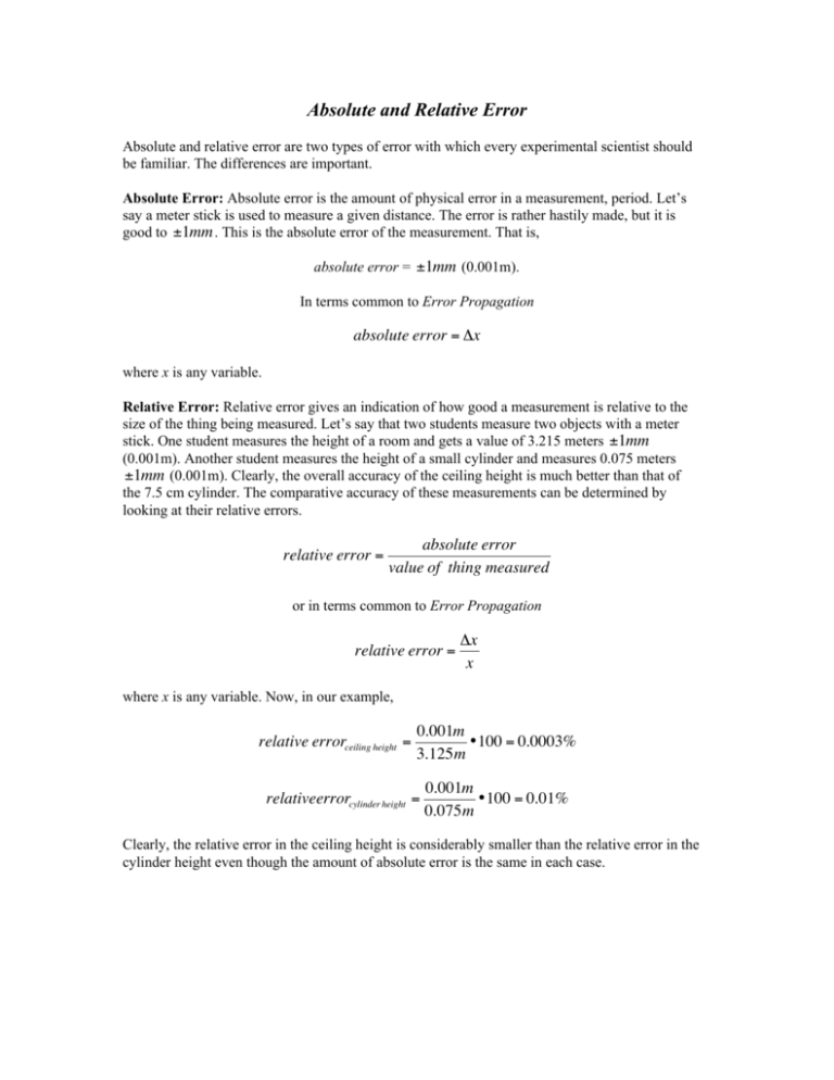
Absolute and Relative Error
Absolute and relative error are two types of error with which every experimental scientist should
be familiar. The differences are important.
Absolute Error: Absolute error is the amount of physical error in a measurement, period. Let’s
say a meter stick is used to measure a given distance. The error is rather hastily made, but it is
good to ±1mm . This is the absolute error of the measurement. That is,
absolute error = ±1mm (0.001m).
€
In terms common to Error Propagation
€absolute error = Δx
where x is any variable.
€ gives an indication of how good a measurement is relative to the
Relative Error: Relative error
size of the thing being measured. Let’s say that two students measure two objects with a meter
stick. One student measures the height of a room and gets a value of 3.215 meters ±1mm
(0.001m). Another student measures the height of a small cylinder and measures 0.075 meters
±1mm (0.001m). Clearly, the overall accuracy of the ceiling height is much better than that of
the 7.5 cm cylinder. The comparative accuracy of these measurements can be determined by
€
looking at their relative errors.
€
relative error =
absolute error
value of thing measured
or in terms common to Error Propagation
€
relative error =
Δx
x
where x is any variable. Now, in our example,
€
0.001m
relative errorceiling height =
•100 = 0.0003%
3.125m
relativeerrorcylinder height =
€
0.001m
•100 = 0.01%
0.075m
Clearly, the relative error in the ceiling height is considerably smaller than the relative error in the
cylinder height even though the amount of absolute error is the same in each case.
€
Errors, Accuracy, and Precision
In making physical measurements, one needs to keep in mind that measurements are not
completely accurate. Each measurement will have some number of significant figures and should
also have some indication as to how much we can “trust” it (i.e. error bars). Thus in order to
reliably interpret experimental data, we need to have some idea as to the nature of the “errors”
associated with the measurements. There are whole text books devoted to error analysis. We will
not even attempt to be complete in our discussion of the topic, rather we will present some basic
ideas to assist you in analyzing your data.
When dealing with error analysis, it is a good idea to know what we really mean by error. To
begin with, let’s talk about what error is not. Error is not a blunder such as forgetting to put the
decimal point in right place, using the wrong units, transposing numbers, or any other silly
mistake. Error is not your lab partner breaking your equipment. Error isn’t even the difference
between your own measurement and some generally accepted value. (That is a discrepancy.)
Accepted values also have errors associated with them; they are just better measurements than
you will be able to make in a three-hour undergraduate physics lab. What we really mean by
error has to do with uncertainty in measurements. Not everyone in lab will come up with the
same measurements that you do and yet (with some obvious exceptions due to blunders) we may
not give preference to one person’s results over another’s. Thus we need to classify types of
errors.
Generally speaking, there are two types of errors: 1) systematic errors and 2) random errors.
Systematic errors are errors that are constant and always of the same sign and thus may not be
reduced by averaging over a lot of data. Examples of systematic errors would be time
measurements by a clock that runs too fast or slow, distance measurements by an inaccurately
marked meter stick, current measurements by inaccurately calibrated ammeters, etc. Generally
speaking, systematic errors are hard to identify with a single experiment. In cases where it is
important, systematic errors may be isolated by performing experiments using different
procedures and comparing results. If the procedures are truly different, the systematic errors
should also be different and hopefully easily identified. An experiment that has very small
systematic errors is said to have a high degree of accuracy.
Random errors are a whole different bag. These errors are produced by any one of a number of
unpredictable and unknown variations in the experiment. Examples might include fluctuations in
room temperature, fluctuations in line voltage, mechanical vibrations, cosmic rays, etc.
Experiments with very small random errors are said to have a high degree of precision.
Since random errors produce variations both above and below some average value, we may
generally quantify their significance using statistical techniques.
Significant Figures in Measurements and Computations
Uncertainty in Measurements: The word accuracy has various connotations depending on the
circumstances under which it is used. In the study of physics it is commonly used to denote the
reliability of a number or the limiting accuracy of a measurement.
As applied to a measurement, the accuracy is expressed by stating the uncertainty of the numerical
result, that is, the estimated maximum amount by which the result may differ from the "true" or
accepted value.
For instance, if we have a keg advertised to contain 15,000 nails, we can assume that there are
between 14,000 and 16,000 nails. The uncertainty amounts to +/- 1 in the last significant figure.
Significant Figures: The accuracy of a physical measurement is properly indicated by the number
of figures used to express the numerical measure. Conventionally, only those figures that are
reasonably trustworthy are retained. These are called significant figures.
In recording certain numbers, the location of the decimal point requires zeros to be added to the
significant figures. These zeros serve only to locate the decimal point and are never considered
significant.
Examples:
Length of a page 22.7 cm (3 significant figures)
Thickness of a page = 0.011 cm (2 significant figures)
Distance to the sun = 149,600,000 km (4 significant fig)
Speed of light = 299,790 km/sec (5 significant figures)
If each of these numbers is expressed in terms of scientific notation, there is no doubt as to the
number of significant figures for only the significant figures are then retained. Thus:
Length of page = 2.27 x 101 cm
Thickness of a page = 1.1 x 10-2 cm
Distance to the sun = 1.496 x 108 km
Speed of light = 2.9979 x 105 km/sec
Do not be confused by the placement of a zero in a string of numbers. For instance, say the land
speed record for a bicycle is 80.13 miles per hour. In this case the zero does more than position the
8, 1, and 3. It indicates that the number is 80, not 79 or 81 miles per hour. A zero imbedded in a
string of significant figures can never itself be considered non-significant. The number 80.13 is
accurate to 4 significant figures.
Further, do not be confused by a zero that is said to be of significance. Something may be measured to
an accuracy of 2.000 units. In this case we know that the measurement is accurate to three decimal
places. That is, the measurement lay somewhere between 2.001 and 1.999.
There are some numbers that, by their definition, may be taken to have an unlimited number of
significant figures. For example, the integer 2 and the irrational number ! in the following
relationship for a circle: circumference = 2!r where r is the radius of a circle.
In calculations there is frequent need to use data that have been recorded without a clear indication of
the number of significant figures. For example, a textbook problem may refer to a "two-kilogram
mass", or in an experiment a student may announce that she has measured a certain distance as "3
meters". In such cases the values with the approximate number of significant figures should be written
from what is know or assumed about the way in which the measurement were made. If the distance
referred to were measured with an ordinary tape measure, the distance might appropriately be written
as 3.0 meters. If the distance were carefully measured with a steel scale accurate to the nearest
millimeter, the distance might be recorded as 3.000 meters. In academic problem work a good rule to
follow is to retain three figures unless there is good reason to decide otherwise.
Recapping: The significant figures in a quantity are the meaningful digits in it. There are several
conventions to keep in mind when dealing with significant figures:
1) Any nonzero digit is a significant digit. Examples: 3.14 has three significant digits and 239.67
has five significant digits.
2) Zeros in between nonzero values are significant digits. Example 20.4 has three significant digits.
3) Zeros to the left of the first nonzero digit are NOT significant. Example: 0.0012 has two
significant digits.
4) For numbers with decimal points, zeros to the right of nonzero digits are significant. Example:
Both 2.0 and 0.0020 have two significant digits.
5) For numbers without decimal points, zeros to the right of nonzero digits may or may not be
significant. Example: 350 may have two or three significant digits. To avoid confusion, use a
decimal point: 350. has three significant digits, 350 has two.
6) The last significant digit in a number should have the same order of magnitude as the
uncertainty. Examples: 3.1415±0.0001; 0.8±0.2
7) The uncertainty should be rounded to one or two significant digits.
Rules for Computation: There is always a pronounced and persistent tendency on the part of
beginners to retain too many figures in a computation. This not only involves too much work but,
worse still, leads to a fictitiously precise result.
The following rules are recommended and will save much time that would otherwise be spent in
calculation. Furthermore, their careful use will result in properly indicated accuracies.
1) In recording the result of a measurement or calculation, one, and only one, doubtful digit is
retained. For instance, a caliper whose finest division is 100-thousandths can produce a
measurement that is accurate to five decimal places at best. i.e. 3.02364.
2) In addition or subtraction, do not carry the result beyond the first column that contains a
doubtful figure. Add all figures and then round (see #4 below) the result. For example:
23.6543
10.01
33.6643
which becomes 33.66
3.4
-2.554
0.846
which becomes 0.8
3) In multiplication and division, carry the result to the same number of significant figures that
there are in that term which has the least number of significant figures. For example:
3.95 x 5.1 = 20.145, rounded to 2 significant figures = 20.
34.2/6.29934 = 5.429140196... becomes upon rounding 5.43
4) When “doing” mathematical manipulations with numbers that have varying numbers of
significant digits, the final result cannot have more significant digits than the least well known
digit. In practice, we will keep all the numbers to their known accuracy through out the
calculation and then round to the number of significant figures at the end. Examples:
2.0*3.14159 = 6.3; 25.001+32.0 = 55.0
5) In dropping figures that are not significant (rounding), the last figure retained should be
unchanged if the following figures dropped are less than half the previous digit. It should be
increased by 1 if the following figures dropped are greater than half the previous digit. If the last
digit dropped is 5, the preceding digit should be left unchanged if it is an even number but
increased by 1 if it is an odd number. For example:
24.5627 rounded to four significant figures becomes 24.56
34.2523 rounded to three significant figures becomes 34.3
3.485 rounded to three significant figures becomes 3.48
7.550 rounded to two significant figures becomes 7.6