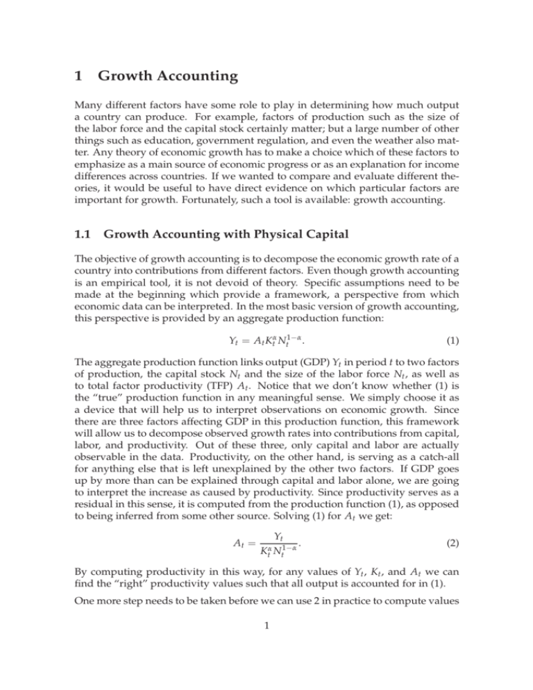
1
Growth Accounting
Many different factors have some role to play in determining how much output
a country can produce. For example, factors of production such as the size of
the labor force and the capital stock certainly matter; but a large number of other
things such as education, government regulation, and even the weather also matter. Any theory of economic growth has to make a choice which of these factors to
emphasize as a main source of economic progress or as an explanation for income
differences across countries. If we wanted to compare and evaluate different theories, it would be useful to have direct evidence on which particular factors are
important for growth. Fortunately, such a tool is available: growth accounting.
1.1 Growth Accounting with Physical Capital
The objective of growth accounting is to decompose the economic growth rate of a
country into contributions from different factors. Even though growth accounting
is an empirical tool, it is not devoid of theory. Specific assumptions need to be
made at the beginning which provide a framework, a perspective from which
economic data can be interpreted. In the most basic version of growth accounting,
this perspective is provided by an aggregate production function:
Yt = At Ktα Nt1−α .
(1)
The aggregate production function links output (GDP) Yt in period t to two factors
of production, the capital stock Nt and the size of the labor force Nt , as well as
to total factor productivity (TFP) At . Notice that we don’t know whether (1) is
the “true” production function in any meaningful sense. We simply choose it as
a device that will help us to interpret observations on economic growth. Since
there are three factors affecting GDP in this production function, this framework
will allow us to decompose observed growth rates into contributions from capital,
labor, and productivity. Out of these three, only capital and labor are actually
observable in the data. Productivity, on the other hand, is serving as a catch-all
for anything else that is left unexplained by the other two factors. If GDP goes
up by more than can be explained through capital and labor alone, we are going
to interpret the increase as caused by productivity. Since productivity serves as a
residual in this sense, it is computed from the production function (1), as opposed
to being inferred from some other source. Solving (1) for At we get:
At =
Yt
Ktα Nt1−α
.
(2)
By computing productivity in this way, for any values of Yt , Kt , and At we can
find the “right” productivity values such that all output is accounted for in (1).
One more step needs to be taken before we can use 2 in practice to compute values
1
for At . Namely, the parameter α enters the computations, and needs to be set in
some fashion. Again, there is no obvious way how α should be chosen. It turns
out, however, that α has a simple interpretation under the additional assumption
that there is perfect competition among firms in the economy. To see this, consider
the profit maximization problem of a firm using production function (1) that rents
capital at rental rate rt and hires labor at wage wt :
α 1−α
A
− rt Kt − wt Nt .
max
t Kt Nt
Kt ,Nt
The first-order conditions for this problem require that the marginal product of
each factor equals its price:
rt =αAt
Nt
Kt
1−α
wt =(1 − α)At
Kt
Nt
,
α
.
Given these expressions, we can compute the capital and labor shares for the economy (the fraction of output used to pay capital and labor, respectively) as:
r t Kt
=α
Yt
wt Nt
= 1 − α.
Labor Share =
Yt
Capital Share =
Therefore, under the assumption of perfect competition the capital share is a measure of the parameter α. The actual capital share for a country is easily found in
national income and product statistics; in most industrialized countries, the capital share is between 0.3 and 0.4, with the labor share varying correspondingly
between 0.6 and 0.7. Once the capital and labor shares have been found, (2) can be
used to compute productivity values for any given year.
We are now ready to proceed to the ultimate goal of decomposing economic growth
into separate contributions from capital, labor, and productivity. Growth rates can
be computed as (natural) log-differences; the growth rate of output in a given year,
for example, can be computed as log Yt+1 − log Yt . Taking logs of the production
function (1) gives:
log Yt = log At + α log Kt + (1 − α) log Nt .
The growth rate of output can therefore be expressed as:
log Yt+1 − log Yt = log At+1 − log At + α (log Kt+1 − log Kt )
+ (1 − α) (log Nt+1 − log Nt ) .
Thus, the growth rate of output equals the growth rate of productivity, plus α
2
times the growth rate of the capital stock, plus 1 − α the growth rate of the labor
force. Intuitively, the impact of any given factor of production on output growth is
proportional to its share in output. Assume, for example, that the capital share is
one-third and the labor share is two-thirds. If the capital stock increased by three
percent in a given year, this growth would translate into just one percent growth
in output. If instead the labor force were to grow by three percent, the resulting
output growth would be two percent. Changes in the labor force have a bigger
impact on output, since labor is more important than capital in production.
Growth accounting can also be carried out if the underlying data come in per
capita or per worker terms. The Penn World Tables, for example, contain information on GDP per worker and the capital stock per worker, but not the size of the
labor force. In this case, the strategy is to transform the production function (1)
into a per-worker production function by dividing by the labor force Nt on both
sides:
α
At Ktα Nt1−α
Kt
Yt
=
= At
.
Nt
Nt
Nt
Using lower-case letters for income and capital per worker (i.e., yt = Yt /Nt and
kt = Kt /Nt ), we have:
(3)
yt = At kαt .
Parallel to the above, productivity can be computed as:
At =
yt
,
kαt
and the growth decomposition is given by:
log yt+1 − log yt = log At+1 − log At + α (log kt+1 − log kt ) ,
that is, growth in output per worker decomposes into productivity growth and
growth in capital per worker.
1.2 Growth Accounting with Human Capital
The growth accounting framework can be extended to assess the role of human
capital for the determination of output and economic growth. Up to this point,
potential human capital differences across countries or over time were subsumed
in the productivity term At (recall that productivity accounts for all sources of
growth which are not explicitly included in the production function). If information on the stock of human capital is available, we can incorporate human capital
into the production function in order to measure its contribution to growth. To
this end, assume that the production function takes the form:
β
Yt = At Ktα Ht Nt
3
1−α−β
.
(4)
Thus, there are now three inputs, physical capital Kt , the size of the labor force Nt ,
and human capital Ht . We maintain the assumption that the production function
is Cobb-Douglas with constant returns to all three inputs combined. Measuring
Ht and determining its share β is not a trivial task. For Ht , usually measures
of schooling levels or years of schooling of the population are used. For β, in
principle one would like to look at the share of skilled labor (as opposed to “raw”
labor) in output. In practice, the distinction between skilled and unskilled labor is
not a sharp one, so that there is no obvious way to determine β.
These problems notwithstanding, assume that measures of Ht and β are available.
Growth accounting now proceeds along the same route as before. Solving (4) for
At results in an implied productivity series:
At =
Yt
.
β
1−α−β
Ktα Ht Nt
(5)
Notice that, despite the fact that the variable has the same name, these productivity values are different than the ones computed in (2), since this time we explicitly
account for the role of human capital.
Based on the computed productivity series, we can apply the same growth breakdown as above to get:
log Yt+1 − log Yt = log At+1 − log At + α (log Kt+1 − log Kt )
+ β (log Ht+1 − log Ht ) + (1 − α − β) (log Nt+1 − log Nt ) .
Thus, the growth rate of output equals the growth rate of productivity, plus α
times the growth rate of the capital stock, plus β times the growth rate of human
capital, plus 1 − α − β the growth rate of the labor force.
Once again, growth accounting can also be carried out if data comes in per-worker
format. The production function (4) can be transformed into a per-worker production function by dividing by the labor force Nt on both sides:
β
1−α−β
At Ktα Ht Nt
Yt
=
Nt
Nt
= At
Kt
Nt
α Ht
Nt
β
.
Using lower-case letters for income, capital, and human capital per worker we
have:
β
yt = At kαt ht .
(6)
The productivity series can be computed as:
At =
yt
β
kαt ht
4
,
and the growth decomposition is given by:
log yt+1 − log yt = log At+1 − log At + α (log kt+1 − log kt )
+ β (log ht+1 − log ht ) .
Using the per-worker production function is often useful, since most data on human capital already comes in a per-person format (such as average years of schooling per person).
5