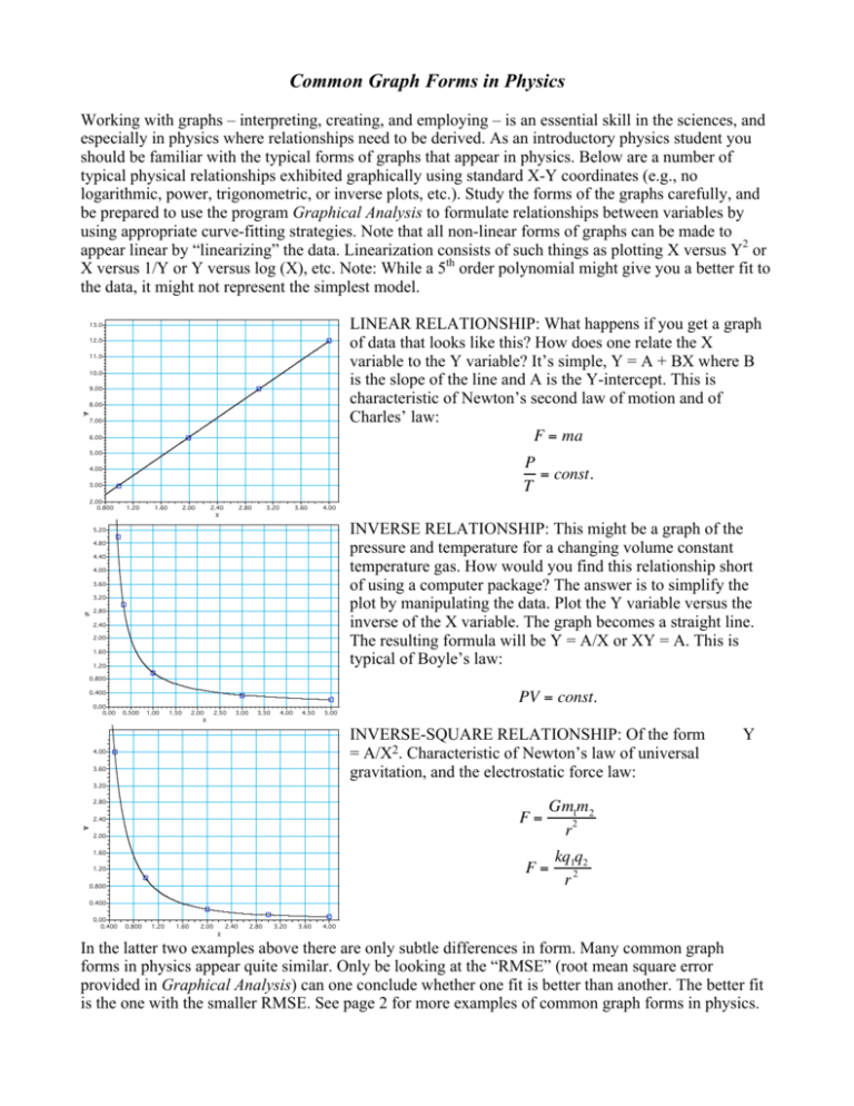
Common Graph Forms in Physics
Working with graphs – interpreting, creating, and employing – is an essential skill in the sciences, and
especially in physics where relationships need to be derived. As an introductory physics student you
should be familiar with the typical forms of graphs that appear in physics. Below are a number of
typical physical relationships exhibited graphically using standard X-Y coordinates (e.g., no
logarithmic, power, trigonometric, or inverse plots, etc.). Study the forms of the graphs carefully, and
be prepared to use the program Graphical Analysis to formulate relationships between variables by
using appropriate curve-fitting strategies. Note that all non-linear forms of graphs can be made to
appear linear by “linearizing” the data. Linearization consists of such things as plotting X versus Y2 or
X versus 1/Y or Y versus log (X), etc. Note: While a 5th order polynomial might give you a better fit to
the data, it might not represent the simplest model.
LINEAR RELATIONSHIP: What happens if you get a graph
of data that looks like this? How does one relate the X
variable to the Y variable? It’s simple, Y = A + BX where B
is the slope of the line and A is the Y-intercept. This is
characteristic of Newton’s second law of motion and of
Charles’ law:
F = ma
13.0
12.0
11.0
10.0
9.00
Y
8.00
7.00
6.00
5.00
P
= const.
T
4.00
3.00
2.00
0.800
1.20
1.60
2.00
2.40
X
2.80
3.20
3.60
4.00
INVERSE RELATIONSHIP: This might be a graph of the
pressure and temperature for a changing volume constant
temperature gas. How would you find this relationship short
of using a computer package? The answer is to simplify the
plot by manipulating the data. Plot the Y variable versus the
inverse of the X variable. The graph becomes a straight line.
The resulting formula will be Y = A/X or XY = A. This is
typical of Boyle’s law:
5.20
4.80
4.40
4.00
3.60
Y
3.20
2.80
2.40
2.00
1.60
1.20
0.800
0.400
0.00
0.00
PV = const.
0.500
1.00
1.50
2.00
X
2.50
3.00
3.50
4.00
4.50
5.00
INVERSE-SQUARE RELATIONSHIP: Of the form
= A/X2. Characteristic of Newton’s law of universal
gravitation, and the electrostatic force law:
4.00
3.60
Y
3.20
2.80
F=
Y
2.40
2.00
Gm1m2
r2
1.60
F=
1.20
0.800
kq1q2
r2
0.400
0.00
0.400
0.800
1.20
1.60
2.00
2.40
2.80
3.20
3.60
4.00
X
In the latter two examples above there are only subtle differences in form. Many common graph
forms in physics appear quite similar. Only be looking at the “RMSE” (root mean square error
provided in Graphical Analysis) can one conclude whether one fit is better than another. The better fit
is the one with the smaller RMSE. See page 2 for more examples of common graph forms in physics.
DOUBLE-INVERSE RELATIONSHIP: Of the form 1/Y = 1/X
+ 1/A. Most readily identified by the presence of an asymptotic
boundary (y = A) within the graph. This form is characteristic of
the thin lens and parallel resistance formulas.
1 1 1
= +
f di d o
1
1
1
=
+
Rt R1 R2
and
€
POWER RELATIONSHIP: Top opening parabola. Of the form Y
= AX2. Typical of the distance-time relationship:
4.00
3.60
3.20
2.80
2.40
Y
d=
2.00
1.60
1 2
at
2
1.20
0.800
0.400
0.00
0.00
0.200
0.400
0.600
0.800
1.00
X
1.20
1.40
1.60
1.80
2.00
POWER RELATIONSHIP: Side opening parabola. Of the form
Y2=A1X or Y=A2X1/2. Typical of the simple pendulum
relationship:
P 2 = k1l or P = k2 l
€
€
POLYNOMIAL OF THE SECOND DEGREE: Of the form Y =
AX + BX2. Typical of the kinematics equation:
13.0
12.0
11.0
10.0
9.00
d = vo t +
8.00
Y
7.00
6.00
1 2
at
2
5.00
4.00
3.00
2.00
1.00
0.00
0.00
0.400
0.800
1.20
1.60
X
2.00
2.40
2.80
3.20
EXPONENTIAL RELATIONSHIP: Of the form
Y=A*
exp(BX). Characteristic of exponential growth or decay. Graph to
left is exponential growth. The graph of exponential decay would
look not unlike that of the inverse relationship. Characteristic of
radioactive decay.
7.60
7.20
6.80
6.40
6.00
5.60
5.20
4.80
Y
4.40
4.00
3.60
N = N oe− λt
3.20
2.80
2.40
2.00
1.60
1.20
0.200
0.400
0.600
0.800
1.00
1.20
1.40
1.60
1.80
2.00
X
€
NATURAL LOG (LN) RELATIONSHIP: Of the form
Y = A ln(BX). Characteristic of entropy change during a free
expansion:
1.80
1.60
1.40
1.20
1.00
0.800
0.600
Y
S f − Si = nRln
0.400
0.200
0.00
-0.200
-0.400
-0.600
-0.800
0.500
1.00
1.50
2.00
2.50
3.00
X
3.50
4.00
4.50
5.00
Vf
Vi