Exploiting the Cost (In)sensitivity of Decision Tree Splitting Criteria Chris Drummond, Robert C. Holte
cdrummon@site.uottawa.ca, holte@site.uottawa.ca
School of Information Technology and Engineering,
University of Ottawa, Ottawa, Ontario, Canada, K1N 6N5
From: AAAI Technical Report WS-00-05. Compilation copyright © 2000, AAAI (www.aaai.org). All rights reserved.
Abstract
This paper investigates how the splitting criteria and pruning
methods of decision tree learning algorithms are influenced
by misclassification costs or changes to the class distribution.
Splitting criteria that are relatively insensitive to costs (class
distributions) are found to perform as well as or better than,
in terms of expected misclassification cost, splitting criteria
that are cost sensitive. Consequently there are two opposite
ways of dealing with imbalance. One is to combine a costinsensitive splitting criterion with a cost insensitive pruning
method to produce a decision tree algorithm little affected
by cost or prior class distribution. The other is to grow a
cost-independent tree which is then pruned in a cost-sensitive
manner.
Introduction
When applying machine learning to real world classification problems two complications that often arise are imbalanced classes (one class occurs much more often than the
other (Kubat, Holte, & Matwin 1998; Ezawa, Singh, & Norton 1996; Fawcett & Provost 1996)) and asymmetric misclassification costs (the cost of misclassifying an example
from one class is much larger than the cost of misclassifying an example from the other class (Domingos 1999;
Pazzani et al. 1997)). Traditional learning algorithms,
which aim to maximize accuracy, treat positive and negative
examples as equally important and therefore do not always
produce a satisfactory classifier under these conditions. Furthermore, in these circumstances accuracy is not an appropriate measure of classifier performance (Provost, Fawcett,
& Kohavi 1998). Class imbalance and asymmetric misclassification costs are related to one another. One way to counteract imbalance is to raise the cost of misclassifying the minority class. Conversely one way to make an algorithm cost
sensitive is to intentionally imbalance the training set.
In this paper we investigate how the splitting criteria of
decision tree learning algorithms are influenced by changes
to misclassification costs or class distribution. We show that
splitting criteria in common use are relatively insensitive to
costs and class distribution; costs and class distribution primarily affect pruning (Breiman et al. 1984, p.94). One criterion, which we refer to as DKM (Kearns & Mansour 1996;
To Appear in the Proceedings of Seventeenth International
Conference on Machine Learning 2000
Dietterich, Kearns, & Mansour 1996) is completely insensitive to costs and class distributions but in our experiments its
performance equals or exceeds that of other splitting criteria.
This suggests two different ways of dealing with imbalance and costs. First, instead of artificially adjusting balance
by duplicating or discarding examples, a cost-insensitive
splitting criterion can be combined with a cost insensitive
pruning method to produce a decision tree algorithm little
affected by cost or prior class distribution. All the data
available can be used to produce the tree, thus throwing
away no information, and learning speed is not degraded due
to duplicate instances. Alternatively one can grow a costindependent tree which is then pruned in a cost-sensitive
manner. Thus the tree need only be grown once, an advantage as growing trees is computationally more expensive
than pruning.
Measuring Cost Sensitivity
We restrict ourselves to two class problems in which the cost
of a misclassification depends only on the class not on the
individual example. Following (Provost & Fawcett 1998) we
use ROC methods to analyze and compare the performance
of classifiers.
One point in an ROC diagram dominates another if it is
above and to the left, i.e. has a higher true positive rate (TP)
and a lower false positive rate (FP). If point A dominates
point B, A will outperform B for all possible misclassification costs and class distributions. By “outperforms” we
typically mean “has lower expected cost”, but (Provost &
Fawcett 1998) have shown that dominance in ROC space implies superior performance for a variety of commonly-used
performance measures.
The slope of the line connecting two ROC points
(FP1 ; TP1 ) and (FP2 ; TP2 ) is given by equation 1
(Provost, Fawcett, & Kohavi 1998; Provost & Fawcett 1997)
TP1 , TP2
FP1 , FP2
=
p(,)C (+j,)
p(+)C (,j+)
(1)
where p(x) is the probability of a given example being
in class x, and C (xjy ) is the cost incurred if an example
in class y is misclassified as being in class x. Equation 1
shows that, for the purpose of evaluating performance in 2class problems, class probabilities (“priors”) and misclassification costs are interchangeable. Doubling p(+) has the
same effect on performance as doubling the cost C (,j+) or
halving the cost C (+j,). In the rest of the paper we will
freely interchange the two, speaking of costs sometimes and
priors other times.
A classifier is a single point in ROC space. Point (0,0) represents classifying all examples as negative, (1,1) represents
classifying all examples as positive. We call these the trivial
classifiers. The slopes of the lines connecting a non-trivial
classifier to (0,0) and to (1,1) define the range of cost ratios
for which the classifier is potentially useful. For cost ratios
outside this range, the classifier will be outperformed by a
trivial classifier. It is important in comparing two classifiers
not to use a cost ratio outside the operating range of one of
them. A classifier's operating range may be much narrower
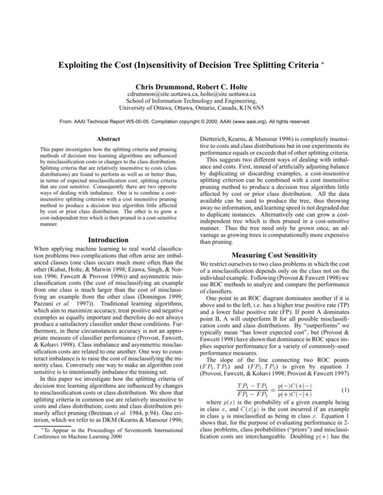
than one intuitively expects. Consider the solid lines in Figure 1. These connect (0,0) and (1,1) to a classifier which
is approximately 70% correct on each class. The slopes,
shown below the lines, are 0.45 and 2.2. If the cost ratio is
outside this range this classifier is outperformed by a trivial
classifier. Operating range increases as one moves towards
the ideal classifier, (0,1). Therefore if classifier A dominates
classifier B, A's operating range will be larger than B's.
1
0.2
0.41
0.9
0.45
0.67
True Positive Rate
0.8
0.7
1
0.6
1.5
0.5
0.4
2.4
2.2
0.3
0.2
4.9
0.1
0
0
0.1
0.2
0.3
0.4
0.5
0.6
0.7
0.8
0.9
1
False Positive Rate
Figure 1: ROC hulls showing line segment slopes
Some classifiers have parameters for which different settings produce different ROC points. For example, a classifier that produces probabilities of an example being in each
class, such as a Naive Bayes classifier, can have a threshold
parameter biasing the final class selection (Domingos 1999;
Pazzani et al. 1997). The upper convex hull (Provost &
Fawcett 1997) of all the ROC points produced by varying
these parameters is the ROC hull for the classifier. The ROC
hull is a discrete set of points, including (0,0) and (1,1), connected by line segments. The dashed line in Figure 1 is a typical ROC hull. The operating range of any point on an ROC
hull is defined by the slopes of the two line segments connected to it. The figure shows the slope below each dashed
line segment. The operating range of a parameterized classifier is the range defined by the two extreme line segments,
the ones involving (0,0) and (1,1). The operating range of
the dashed ROC hull in the figure is about 1:14 to 14:1.
The cost-sensitivity of a classifier can be defined in terms
of its ROC hull, for example, as the length of the ROC hull
not counting the lines to (0,0) and (1,1). This measures the
amount of variation in performance that can be achieved
by varying the classifier's parameters. An unparameterized
classifier is not cost-sensitive at all according to this definition. Alternatively cost-sensitivity could be defined as
the size of the classifier's operating range. This definition
measures the range of cost ratios for which the classifier is
useful. Both definitions give important information about
a classifier when costs or priors are not known in advance,
but they can give opposite conclusions about which of two
classifiers is more cost-sensitive because it is possible for
classifier A to have a much shorter ROC hull than B but to
have a larger operating range. This happens, for example, if
A dominates B. The most striking example is when A is an
unparameterized classifier whose performance is sufficiently
good that its ROC hull completely dominates B's ROC hull.
For example, the ROC hull of an unparameterized classifier that was 94% correct on each class would dominate the
dashed ROC hull in Figure 1.
A learning algorithm may produce different classifiers
when its parameters' values are changed or when the class
distribution in the training set is changed while keeping all
the conditional probabilities within each class the same. For
example, the ROC hull in Figure 1 was generated by applying the same learning algorithm to training sets in which
the class ratio was artificially varied. The stipulation that
the within-class conditional probabilities must not change is
important. It can be achieved exactly by duplicating all the
examples in one of the classes the same number of times
(“oversampling”), and it can be approximately achieved by
choosing a random subset of the examples in one class (“undersampling”). The cost-sensitivity of a learning algorithm
can be measured in several ways. It could be defined in
terms of the responsiveness of the learning algorithm to
changes in the class distribution as measured, for example,
by the length of the ROC hull produced when the class ratio
in the training set is varied between two extremes (e.g. 1:10
to 10:1). Alternatively, it could be defined “structurally”, as
the degree to which the classifiers produced differ from one
another when costs or priors are varied.
None of these definitions of cost-sensitivity is directly related to performance. System A can be more cost-sensitive
than system B according to any of the definitions and yet be
outperformed by B on almost their entire operating range.
Performance is our ultimate criterion for preferring one system over another. Cost-sensitivity is only desirable if it produces improved performance, it is not a goal in itself.
To directly compare performance we transform an ROC
hull into a cost curve (see (Drummond & Holte 2000) for
a detailed discussion of cost curves). Figure 2 shows three
cost curves. The x-axis is p(+), the prior probability of the
positive class. The y-axis is expected cost normalized with
respect to the cost incurred when every example is incorrectly classified. The classifier that classifies everything as
belonging to the majority class has an expected normalized
cost of 0.5 when p(+) = 0:5 and its expected cost decreases
Cost Sensitivity of the Split Criteria
This section investigates how different class distributions affect the four different splitting criteria shown in Figure 3.
The triangular function represents accuracy. Immediately
above that is the Gini criterion used in CART (Breiman et
al. 1984), followed by information gain or entropy as used
in C4.5 (Quinlan 1996). At the top is the criterion we call
DKM (Kearns & Mansour 1996; Dietterich, Kearns, & Mansour 1996). The splitting criteria all have the same general
form. The selected split is the minimum of I (s) the total
impurity after applying the split, as shown in equation 2.
I (s) = P (L)f (P (+jLs); P (,jLs ))
+P (R)f (P (+jRs ); P (,jRs ))
(2)
Normalised Misclassification Costs
DKM
Entropy
0.8
Gini
0.7
Accuracy
0.6
0.5
0.4
0.3
0.2
0.1
0
0
0.1
0.2
0.3
0.4
0.5
0.6
0.7
0.8
0.9
1
Probability of Positive Class
Figure 3: Decision Tree Splitting Criteria
perfect knowledge of the conditional probabilities and the
priors. The conditional probabilities for the two classes are
Gaussians with the same standard deviation but with means
one standard deviation apart. By changing the priors on one
of the Gaussians, as indicated by the dashed lines in Figure
4, different Bayes optimal splits are achieved.
Figure 4: A Simple Decision Problem
The accuracy criterion, which uses the impurity function
f (a; b) = min(a; b), produces Bayes optimal splits in this
0.5
0.45
0.4
0.35
0.3
0.25
0.2
0.15
0.1
0.05
0
1
0.9
Impurity
linearly towards 0 as the probability of the majority class increases. Its cost curve is the dotted line in Figure 2. The
dashed and solid cost curves in Figure 2 correspond to the
dashed and solid ROC hulls in Figure 1. The horizontal line
atop the solid cost curve corresponds to the unparameterized classifier. The location of the line indicates the classifier's operating range (0:3 p(+) 0:7). It is horizontal
because FP = 1 , TP for this classifier. At the limit of
its operating range this classifier's cost curve joins the cost
curve for the majority classifier. Each line segment in the
dashed cost curve corresponds to one of the vertices defining the dashed ROC hull. The difference in performance of
two classifiers is precisely the difference between their cost
curves. The dashed classifier outperforms the solid one –
has a lower or equal expected cost – for all values of p(+).
The maximum difference is about 20% (0.25 compared to
0.3), which occurs when p(+) is about 0:3 (or 0:7).
0
0.1
0.2
0.3
0.4
0.5
0.6
0.7
0.8
0.9
1
Probability of Positive Class
Figure 2: Cost curves for the ROC hulls in Figure 1
This is the weighted sum of an impurity function f (a; b)
applied to the posterior probabilities of each class for each
side of the split. The weights are the probability of an example going to the left P (L) or right P (R) of the split. The
exact shape of each curve in Figure 3 is determined by the
impurity function.
To investigate the cost sensitivity of the splitting criteria,
we synthesize a simple single attribute problem and assume
synthetic problem. The top diagram in Figure 5 shows the
splits selected for cost ratio from about 10/1 to 1/10 moving
from the bottom to the top. Examples are classified as positive in the shaded regions, and as negative in the unshaded
regions.
The second diagram in Figure 5, shows the splits made
using the Gini criterion where f (a; b) is 2ab. The difference
in the position of the split as the ratio is changed is much
smaller than for accuracy and therefore the Bayes optimal.
For the more extreme ratios, although a split has occurred,
the classification on both the left and right sides is the same.
The third diagram in Figure 5 shows the splits made using
the entropy criterion where f (a; b) is a log2 (a) + b log2 (b).
The splits for all the ratios are very similar, showing that
entropy has little sensitivity to priors. Finally, the bottom diagram in Figure 5 shows thatpthe splits made using the DKM
criterion, where f (a; b) is 2 ab, are identical for all ratios.
Appendix presents a simple proof that DKM is completely
insensitive to cost/priors.
The sensitivity to cost of the various splitting criteria thus
follows the order, from accuracy to DKM, in which they appear in Figure 3, with accuracy being extremely cost sensitive and DKM being totally insensitive. Accuracy and DKM
ACCURACY
Ratio
10.2:1
+
1:10.2
+
+
GINI
-
ENTROPY
10.2:1
-
1:10.2
+
+
+
-
+
+
+
DKM
1:10.2
-
-
+
+
+
-
10.2:1
-
-
-
10.2:1
1:10.2
+
-
-
+
+
+
-
on the same data its ROC hull is virtually indistinguishable
from the hull reported here for the entropy criterion.
Twelve different cost ratios were used, ranging from 1:60
to 60:1. The cost ratios are introduced by reducing the individual weights of instances of the less costly class in proportion to its ratio to the more costly one. This is done in the
C4.5 code that builds and that prunes the tree. For each ratio
we repeated 10-fold stratified cross validation ten times and
averaged the resulting false positive rates and true positive
rates to get a single (FP; TP ) point. The twelve ratios thus
produce twelve ROC points for a given splitting criterion.
600
Accuracy
400
200
-3
-2
-1
0
1
2
3 SD
0
0
1
2
3
4
5
6
7
8
9
10
11
12
13
1
2
3
4
5
6
7
8
9
10
11
12
13
2
3
4
5
6
7
8
9
10
11
12
13
2
3
4
5
6
7
8
9
10
11
12
13
600
Figure 5: Decision Boundaries
Gini
400
200
0
represent the two limits of useful splitting criteria. Going
below accuracy would produce functions that are no longer
concave and therefore not useful as splitting criteria. Going
above DKM would produce functions that have an inverse
sensitivity to cost.
The preceding discussion concerns “structural” sensitivity, i.e., how much the split changes when priors change.
The other notions of sensitivity introduced in section follow the same pattern. The curves in Figures 1, and 2 are
the results of this experiment for accuracy (dashed curves)
and DKM (solid curves). On this problem the more costsensitive the splitting criterion the better the performance
and the wider the operating range. As discussed in section
accuracy's expected cost is up to 20% smaller than DKM's.
0
600
Entropy
400
200
0
0
1
600
DKM
400
200
0
0
1
Figure 6: Consistency
1
5.1
0.9
The Split Criteria on Real Data
0.8
5.1
0.7
True Positive Rate
On 1-dimensional Gaussian data accuracy produces the
Bayes optimal split. But with multiple attributes the optimal
decision boundary is much more complicated and accuracy
is often not the best criterion for growing a tree (Breiman et
al. 1984, p97). This section investigates the cost-sensitivity
and performance of the splitting criteria on real data. Two
of the data sets used, oil and sleepbr2, are from our earlier
work (Kubat, Holte, & Matwin 1997) and one, appendicitis, was supplied by S. Weiss of Rutgers University. Three
additional sets were taken from the UCI collection (Blake
& Merz 1998): Pima diabetes, sonar were used unchanged;
glass was converted to a two class problem by combining
the classes in the “float” and “non-float” groups.
Decision trees were built using C.45 release 8 (Quinlan
1996) in which we disabled the additional penalty factor for
continuous variables based on minimum description length
and we set the minimum size of a split equal to 2 independent of the number of instances. The four splitting criteria
from section were used in place of the normal one. These
changes were made so that the cost-sensitivity and performance of the four criteria could be measured without confounding factors. If the unmodified C4.5 release 8 is run
0.6
0.2
0.5
0.4
0.3
DKM
ACC
0.2
0.2
0.1
0 0.017
0
0.1
0.2
0.3
0.4
0.5
0.6
0.7
0.8
0.9
1
False Positive Rate
Figure 7: Diabetes Unpruned
Figure 6 shows the consistency in the choice of the root
attribute/value for each splitting criterion. Consistency was
measured as follows. For each fold of each repetition of
cross-validation on each dataset, we count how many times
the same root attribute/value is chosen when using different
cost ratios. For example, if one attribute/value was chosen
for 5 of the ratios, another attribute/value was chosen for
1
pruning to adjust for costs. In the other data sets there is less
chance for pruning to have this effect.
This section has shown that DKM is cost-insensitive in
terms of the decision trees it constructs and its responsiveness to variation in cost ratio. Although cost-insensitive in
these other senses, it is possible that DKM might be more
cost-sensitive than the other criteria in terms of the size of
its operating range and it might outperform them in terms of
expected cost.
5.1
5.1
0.9
0.8
True Positive Rate
0.7
0.6
0.5
0.4
0.2
0.3
0.2
DKM
ACC
0.2
1
0.9
0.1
0.8
0.1
0.2
0.3
0.4
0.5
0.6
0.7
0.8
0.9
1
False Positive Rate
Figure 8: Diabetes Pruned
another 5 of the ratios, and a third attribute/value was chosen for the other 2 ratios, we would record this as the bag
f5; 5; 2g. The same attribute/value being chosen for all the
ratios is the bag f12g and a different attribute/value being
chosen for each ratio is the bag containing twelve ones. The
bag is reduced to a single number, the consistency score for
that particular training set, by summing the squares of its
values and dividing by 12. For example, f5; 5; 2g produces
a consistency score of 54=12 = 4:5. This method for computing consistency is somewhat arbitrary in its details but it
has the important properties that the maximum score (12)
occurs only if the same root attribute/value is chosen for all
the ratios, the minimum score (1) occurs only if each ratio results in a different root attribute/value being selected,
and it generally agrees with the intuitive judgements of relative consistency in clearcut cases (for example the score for
f6; 6g is considerably higher than the score for f4; 4; 4g).
For each splitting criterion, our complete set of experiments produces 600 scores (1010 folds for 6 datasets). The
histogram for a splitting criterion in Figure 6 uses integer
bins to summarize these scores. DKM is almost perfectly
consistent choosing the same attribute/value nearly every
time. With entropy, the consistency depends on the data
set, ranging from mostly choosing the same attribute/value
to choosing different ones for different ratios. Gini and particularly accuracy choose different attribute/values for many
of the ratios. Thus the root of the tree is consistent for DKM
but is very dependent on the ratio for accuracy. Figure 7
shows the range of points generated by the middle eight of
the twelve ratios using an unpruned decision tree on the diabetes data set. The limits of this range are indicated by the
numbers. The dashed line is accuracy, points are well spread
out across ROC space. For DKM the spread is much narrower, consistent with a low structural cost sensitivity. However when the tree is pruned (Figure 8) the size of spread
is increased considerably, until there is relatively little difference between the end points of the range. Roughly the
same behavior is exhibited on all the data sets, but the effect
of pruning is often much reduced. C4.5 grows a large tree
on the diabetes data which gives it many opportunities for
0.7
True Positive Rate
0
0.6
0.5
0.4
0.3
DKM
ENT
GINI
ACC
0.2
0.1
0
0
0.1
0.2
0.3
0.4
0.5
0.6
0.7
0.8
0.9
1
False Positive Rate
Figure 9: ROC Hulls for Appendicitis
1
0.9
0.8
0.7
True Positive Rate
0
0.6
0.5
0.4
0.3
DKM
ENT
GINI
ACC
0.2
0.1
0
0
0.1
0.2
0.3
0.4
0.5
0.6
0.7
0.8
0.9
1
False Positive Rate
Figure 10: ROC Hulls for Sleepbr2
Figures 9 to 14 show the ROC hulls for the splitting criteria on the 6 data sets. The ROC hulls are generated by taking the convex hull of the twelve points, one for each of the
twelve ratios, and the two points representing the trivial classifiers. Points not on the hull are discarded. The solid back
diagonal line, FP = 1 , TP , will be discussed in section
. Only in Figure 9 does DKM's insensitivity to cost result
in inferior performance. It dominates when the cost ratio
is extremely high in favor of the negative class (the bottom
left portion of the ROC hull) but fails to adapt as the ratio
decreases. Accuracy, the most cost-sensitive of the criteria,
produces the best performance once DKM stops adapting. In
1
1
0.9
0.9
0.8
0.8
True Positive Rate
0.7
True Positive Rate
0.7
0.6
0.5
0.4
0.3
0.1
0
0
0.1
0.2
0.3
0.4
0.5
0.6
0.5
0.4
0.3
DKM
ENT
GINI
ACC
0.2
DKM
ENT
GINI
ACC
0.2
0.6
0.1
0
0.7
0.8
0.9
1
0
0.1
0.2
0.3
0.4
0.5
0.6
0.7
0.8
0.9
1
False Positive Rate
False Positive Rate
Figure 14: ROC Hulls for Sonar
Figure 11: ROC Hulls for Diabetes
Figures 10 and 11 the criteria all perform about equally well,
with the more cost-sensitive criteria slightly outperforming
DKM in Figure 10. In the remaining three data sets, DKM is
clearly the criterion of choice. In Figure 12 the criteria perform about the same when the cost ratio is extremely high
in favor of the negative class, but DKM emerges to dominate the others once the ratio has swung to favor the positive
class. Figures 13 and 14 are the most striking because there
cost-sensitivity is clearly a disadvantage, with performance
being inversely related to cost sensitivity.
1
0.9
0.8
True Positive Rate
0.7
0.6
0.5
0.4
Discussion
0.3
DKM
ENT
GINI
ACC
0.2
0.1
0
0
0.1
0.2
0.3
0.4
0.5
0.6
0.7
0.8
0.9
1
0.9
1
False Positive Rate
Figure 12: ROC Hulls for Oil
1
0.9
0.8
True Positive Rate
0.7
0.6
0.5
0.4
0.3
DKM
ENT
GINI
ACC
0.2
0.1
0
0
0.1
0.2
0.3
0.4
0.5
0.6
0.7
0.8
False Positive Rate
Figure 13: ROC Hulls for Glass2
In these figures DKM is the combination of a costinsensitive splitting criterion (DKM) and cost-sensitive
pruning and leaf-labeling methods. We have seen that this
combination generally performs as well as or better than using a cost-sensitive splitting criterion with the same pruning
and leaf-labeling methods. The fact that the splitting can
be done independently of cost/priors has several interesting
consequences. In applications where a classifier is to be deployed at several sites with different costs/priors, the same
tree can be grown using DKM and distributed to all sites.
Each site can then prune the tree to suit its local conditions.
Moreover, if attributes are measured only when needed, and
the true classifications of the examples classified by the tree
eventually become known, these examples can be used for
pruning even though they could not be used to learn a new
tree from scratch because they have so few measured attributes. The structural stability of the cost-insensitive tree
is important for comprehensibility. Experts analyzing the
tree can be assured that the attribute and value defining the
split at the root node is a stable feature of the tree, not something that is highly sensitive to the training data. More generally, the fact that good decision trees can be grown in a
cost-insensitive way suggests that research should focus on
ways of making classifiers cost-sensitive, rather than learners. Techniques such as under- and oversampling (Kubat &
Matwin 1997) should be reconsidered in terms of how they
affect pruning and leaf labeling, which can be regarded as
ways of adapting a classifier (fully grown decision tree) to
varying costs and priors.
to increase the overall misclassification costs by a relatively
small amount.
0.35
References
Normalised Misclassification Costs
0.3
0.25
0.2
0.15
0.1
DKM
ENT
GINI
ACC
0.05
0
0
0.1
0.2
0.3
0.4
0.5
0.6
0.7
0.8
0.9
1
Probability of Positive Class
Figure 15: Cost Curves for Sonar
One can even question if cost-sensitive pruning is beneficial. In section a single classifier, combined with the trivial classifiers, was close to Bayes optimal performance over
much of its operating range. The intersection of an ROC
curve with the line FP = 1 , TP (the solid back diagonal
line in Figures 9 to 14) represents a classifier with a normalized expected cost that is totally independent of misclassification costs and priors. Figure 15 shows cost curves for the
different splitting criteria on the sonar data set. For a given
splitting criterion the classifier corresponding to the intersection would be a horizontal line through the highest point
on the cost curve. In all cases this cost-insensitive classifier
has a normalized misclassification cost within 20% of the
basic cost curve and is typically much closer.
A cost-insensitive learning system could also be created by using DKM in conjunction with a cost-insensitive
pruning method. We made C4.5's pruning method costinsensitive by adjusting the instance weights prior to pruning so that total weight for each class was the same. The
cost curve for this algorithm is the solid almost-horizontal
line just above DKM's cost curve in Figure 15. This costinsensitive learning algorithm outperforms algorithms using
the accuracy and Gini splitting criterion and its performance
is similar to the entropy-based learning algorithm for much
of its operating range. It is, however, outperformed by DKM
with cost-sensitive pruning by a little over 25% in some regions of its operating range but in other regions it is much
less.
Conclusions
We have shown that commonly used decision tree splitting
criteria are relatively insensitive to cost. That in fact, a newly
introduced criterion is completely cost insensitive. But as we
have stressed it is performance of the classifier with respect
to costs that is the critical measure. This can only be truly
judged by using ROC hulls or our own direct representation
of misclassification costs. On this basis using a cost insensitive splitting criterion, requiring pruning to introduce any
cost sensitivity, is surprisingly effective. Using a classifier
with a cost insensitive pruning algorithm was also shown
Blake, C. L., and Merz, C. J. 1998. Uci repository of machine learning databases, university of california, irvine, ca
.
www.ics.uci.edu/mlearn/MLRepository.html.
Breiman, L.; Friedman, J. H.; Olshen, R. A.; and Stone,
C. J. 1984. Classification and Regression Trees. Belmont,
CA: Wadsworth.
Dietterich, T. G.; Kearns, M.; and Mansour, Y. 1996. Applying the weak learning framework to understand and improve c4.5. In Proceedings of the Thirteenth International
Conference on Machine Learning, 96–104. San Francisco:
Morgan Kaufmann.
Domingos, P. 1999. Metacost: A general method for making classifiers cost-sensitive. In Proceedings of the Fifth International Conference on Knowledge Discovery and Data
Mining, 155–164. Menlo Park, CA: AAAI Press.
Drummond, C., and Holte, R. C. 2000. Explicitly representing expected cost: An alternative to ROC representation. Technical Report TR-00-02, School of Information
Technology and Engineering, University of Ottawa, Ottawa, Ontario, Canada.
Ezawa, K. J.; Singh, M.; and Norton, S. W. 1996. Learning goal oriented bayesian networks for telecommunications management. In Proceedings of the Thirteenth International Conference on Machine Learning, 139–14. San
Francisco: Morgan Kaufmann.
Fawcett, T., and Provost, F. 1996. Combining data mining and machine learning for effective user profiling. In
Proceedings of the Second International Conference on
Knowledge Discovery and Data Mining, 8–13. Menlo
Park, CA: AAAI Press.
Kearns, M., and Mansour, Y. 1996. On the boosting ability
of top-down decision tree learning algorithms. In Proceedings of the Twenty-Eighth ACM Symposium on the Theory
of Computing, 459–468. New York: ACM Press.
Kubat, M., and Matwin, S. 1997. Addressing the curse of
imbalanced training sets: One-sided selection. In Proceedings of the Fourteenth International Conference on Machine Learning, 179–186. San Francisco: Morgan Kaufmann.
Kubat, M.; Holte, R. C.; and Matwin, S. 1997. Learning when negative examples abound: One-sided selection.
In Proceedings of the Ninth European Conference on Machine Learning, 146–153. Berlin: Springer-Verlag.
Kubat, M.; Holte, R. C.; and Matwin, S. 1998. Machine
learning for the detection of oil spills in satellite radar images. Machine Learning 30:195–215.
Pazzani, M.; Merz, C.; Murphy, P.; Ali, K.; Hume, T.; and
Brunk, C. 1997. Reducing misclassification costs. In Proceedings of the Eleventh International Conference on Machine Learning, 217–225. San Francisco: Morgan Kaufmann.
Provost, F., and Fawcett, T. 1997. Analysis and visualization of classifier performance: Comparison under imprecise class and cost distributions. In Proceedings of the
Third International Conference on Knowledge Discovery
and Data Mining, 43–48. Menlo Park, CA: AAAI Press.
Provost, F., and Fawcett, T. 1998. Robust classification systems for imprecise environments. In Proceedings of the Fifteenth National Conference on Artificial Intelligence, 706–
713. Menlo Park, CA: AAAI Press.
Provost, F.; Fawcett, T.; and Kohavi, R. 1998. The case
against accuracy estimation for comparing induction algorithms. In Proceedings of the Fifteenth International Conference on Machine Learning, 43–48. San Francisco: Morgan Kaufmann.
Quinlan, J. R. 1996. Improved use of continuous attributes
in c4.5. Journal of Artificial Intelligence Research 4:77–
90.
DKM's Independence of Priors
Equation 3 is the general splitting criterion using the DKM
impurity function We replace the posterior probabilities using Bayes rule producing equation 4. The probability of going left, P (L), that weights the first term cancels with the
denominators inside the square root, as does P (R), producing equation 5. Now the prior probabilities P (+) and P (,)
can be brought outside the brackets and being common to
both terms becomes a scaling factor, as shown in equation 6.
In this form it can be seen that the position of the best split,
the minimum of this function, is independent of the prior
probabilities.
I (s)
=
+
=
+
=
+
=
+
P (L)(P (Ls j+)P (Ls j,))1=2
P (R)(P (Rs j+)P (Rs j,))1=2
(3)
P (L)( P (+PjL(sL)P) (+) P (,jPL(sL)P) (,) )1=2
P (R)( P (+PjR(sR)P) (+) P (,jPR(sR)P) (,) )1=2(4)
1=2
(P (+jLs )P (+)P (,jLs )P (,))
1=2
(5)
(P (+jRs )P (+)P (,jRs )P (,))
1=2
1=2
(P (+)P (,))
((P (+jLs ); P (,jLs ))
1=2
(P (+jRs )P (,jRs ))
)
(6)