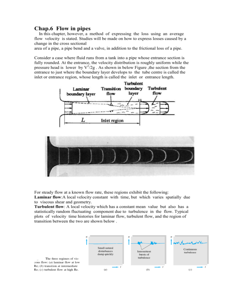
Chap.6 Flow in pipes
In this chapter, however, a method of expressing the loss using an average
flow velocity is stated. Studies will be made on how to express losses caused by a
change in the cross sectional
area of a pipe, a pipe bend and a valve, in addition to the frictional loss of a pipe.
Consider a case where fluid runs from a tank into a pipe whose entrance section is
fully rounded. At the entrance, the velocity distribution is roughly uniform while the
pressure head is lower by V2/2g . As shown in below Figure ,the section from the
entrance to just where the boundary layer develops to the tube centre is called the
inlet or entrance region, whose length is called the inlet or entrance length.
For steady flow at a known flow rate, these regions exhibit the following:
Laminar flow:A local velocity constant with time, but which varies spatially due
to viscous shear and geometry.
Turbulent flow: A local velocity which has a constant mean value but also has a
statistically random fluctuating component due to turbulence in the flow. Typical
plots of velocity time histories for laminar flow, turbulent flow, and the region of
transition between the two are shown below .
Principal parameter used to specify the type of flow regime is the Reynolds number :
V - characteristic flow velocity
D - characteristic flow dimension
μ- dynamic viscosity
υ- kinematic viscosity
We can now define the critical or transition Reynolds number Recr
Recr is the Reynolds number below which the flow is laminar, above which the flow
is turbulent
While transition can occur over a range of Re, we will use the following for internal
pipe or duct flow:
Typical criteria for the length of the entrance region are given as follows:
Le = length of the entrance region .The wall shear is constant, nd the pressure
drops linearly with x,for either laminar or turbulent flow.All these details are shown
in the below Figure
Laminar flow:
computation by Boussinesq
experiment L = 0.065Red by Nikuradse
L = O.06Red computation by Asao, Iwanami and Mori
Turbulent flow:
L = 0.693Re1I4d computation by Latzko
L = (25 - 40)d experiment by Nikuradse
Developing pressure changes in the entrance of a duct flow
Velocity distribution of Laminar Flow in pipe:
In the case of axial symmetry, when cylindrical coordinates are used , the momentum
equation become as following :
---(1)
---- (2)
For the case of a parallel flow like this, the Navier-Stokes equation is extremely
simple as follows:
1. As the velocity is only u since v = 0, it is sufficient to use only the upper
2. As this flow is steady, u does not change with time, so ∂u/∂t = 0.
3. As there is no body force, ρX = 0.
4. As this flow is uniform, u does not change with position, so ∂ul∂x = 0 and
∂2u/∂x2=0
5. Since v= 0, the equation 2 simply expresses the hydrostatic pressure variation and has
no influence in the x direction. So, equation 1 becomes :
Integrating
According to the boundary conditions, since the velocity at r = 0 must be finite c1 =
0 and c2 is determined when u = 0 at r = ro:
Laminar flow in a circular pipe
From this equation, it is clear that the velocity distribution forms a paraboloid of
revolution with umax at r = 0 :
The volumetric flow rate passing pipe Q becomes :
From this equation, the mean velocity v is :
The shear stress due to the viscosity is :
(Since duldr < 0, T is negative, i.e. leftward.) Thus :
Putting the pressure drop in length L as ∆p, the following equation is obtained :
( Hagen-Poiseuille formula )
Using this equation, the viscosity of liquid can be obtained by measuring the pressure
drop ∆p.
Velocity distribution between parallel plates:
Let us study the flow of a viscous fluid between two parallel plates as shown in
below Figure , where the flow has just passed the inlet length. The momentum
equations in x and y directions as in the following :
-------------( 1 )
-------------( 2 )
Under the same conditions as in the previous section , the upper equation (1)
becomes
:
Consider the balance of forces acting on the respective faces of an assumed
small volume
dx dy (of unit
width) in a
fluid.
Since there is no change of momentum between the two faces, the following
equation is obtained:
therefore
By integrating the above equation twice about y, the following equation is obtained:
---------(3)
Using u = 0 as the boundary condition at y = 0 and h, c1 and c2 are found as follows:
It is clear that the velocity distribution now forms a parabola. At y = h/2 , du/dy
= 0 , so u
becomes umax :
The volumetric flow rate Q becomes :
---------(4)
From this equation, the mean velocity v is :
The shearing stress z due to viscosity becomes :
Putting L as the length of plate in the flow direction and ∆p as the pressure
difference, and integrating in the x direction, the following relation is obtained:
Substituting this equation into eqn (4) gives :
As shown in the below Figure , in the case where the upper plate moves in the x
direction at constant speed U or -U, from the boundary conditions of u = 0 at y = 0
and u = U at y = h, c1 and c2 in eqn (3) can be determined. Thus :
and
CouettePoiseuille
flow
Velocity
distribution of turbulent Flow
For two-dimensional flow, the velocity is expressed as follows:
where u and v are the timewise mean velocities and u' and v' are the fluctuating
velocities.
Now, consider the flow at velocity u in the x direction as the flow between two
flat plates as shown in the below Figure , so u = |u| + |u'| but v = v' .
The shearing stress τ of a turbulent flow is :
τ1 = laminar flow shear stress
τt= turbulent shearing where numerous rotating eddies mix
with each other. stress
Now, let us examine the turbulent shearing stress only. The fluid which passes in
unit time in the y direction through dA parallel to the x axis is ρv' dA. Since this
fluid is at relative velocity u' , the momentum is pv' dA u'. By the movement of this
fluid, the upper fluid increases its momentum per unit area by ρ u' v' in the
positive direction of x per unit time.Therefore, a shearing stress develops on face
dA. It is found that the shearing stress due to the turbulent flow is proportional to ρ
u' v' . Reynolds .Thus
Below Figure shows the shearing stress in turbulent flow between parallel flat plates. Expressing
the Reynolds stress as follows as in the case of laminar flow
produces the following as the shearing stress
in
turbulent flow:
This vt is called the turbulent kinematic
viscosity.
Vt is not the value of a physical property dependent
on the temperature or such, but a quantity fluctuating
according to the flow condition.
Prandtl assumed the following equation in which, for rotating small parcels of fluid of turbulent
flow (eddies) traveling average length, the eddies assimilate the character of other eddies by
collisions with them:
Prandtl called this I the mixing length.
According to the results of turbulence measurements
for shearing flow, the distributions of u' and v' are as
shown in the Figure , where u' v' has a large probability
----------(1)
Assuming ‫ ז‬to be the shearing stress acting on the wall, then so far as this section is concerned:
and
=
(
friction of velocity)
Putting u = uδ whenever y=yδ gives
------(2)
where Rδ is a Reynolds number.
Next, since turbulent flow dominates in the neighborhood of the wall
beyond the viscous sublayer, assume ‫ז‬o=‫ז‬t , and integrate eqn (1):
Using the relation ū = uδ when y =δo ,
Using the relation in eqn (2),
If ū/ν‫ ٭‬, is plotted against log10 (ν,y/ν), the value A can be obtained , A = 5.510
This equation is considered applicable only in the neighbourhood of the wall from the
viewpoint of its derivation. In additional, Prandtl separately derived through
experiment the following equation of an exponential function as the velocity
distribution of a turbulent flow in a circular pipe as shown in beow Figure :
n changes according to Re , and is 7 when
Re = 1* 105. Since many cases are generally for
flows in this neighbourhood, the equation where
n = 7 is frequently used.
Losses By pipe Friction
Let us study the flow in the region where the velocity distribution is fully
developed after passing through the inlet region as shown below . If a fluid is
flowing in the round pipe of diameter d at the average flow velocity v, let the
pressures at two points distance L apart be p1 and p2 respectively. The relationship
between the velocity u and the loss head h = ( p 1 - p2 ) /pg For the laminar flow,
the loss head h is proportional to the flow velocity v while for the turbulent
flow, it turns out to be proportional to v1.75-2 .
The loss head is expressed by the following equation as shown in this equation :
This equation is called the Darcy-Weisbach equation', and the coefficient f is called
the friction coefficient of the pipe.
Pipe frictional loss
Relationship between flow
velocity and loss head
Laminar flow
In this case the equations
and
f=
No effect of wall roughness is seen. The reason is probably that the flow turbulence caused by
the wall face coarseness is limited to a region near the wall face because the velocity and
therefore inertia are small, while viscous effects are large in such a laminar region.
Turbulent flow
f generally varies according to Reynolds number and the pipe wall roughness.
Smooth circular pipe
The roughness is inside the viscous sub layer if the height ε of wall face ruggedness
is
In the case of a smooth pipe, the following equations have been developed:
f
f
f
f
f
f
Re√f
f
f
Rough circular pipe
If
whenever Re > 900(ε/d) , it turns out that
f
f
A good approximate equation for the turbulent region of the Moody chart
is given
by Haaland’s equation:
For a new commercial pipe , f can be easily obtained from Moody diagram
shown in Fig.a using ε/d in Fig.b .
Fig,a Mody diagram
f
f
√f
Fig,b
Re√f
Example ( Laminar flow):
Water, ρ=998 kg/m3 ,  = 1.005 ×10-6 m2 /s
flows through a 0.6 cm tube diameter, 30 m
long, at a flow rate of 0.34 L/min. If the pipe
discharges to the atmosphere, determine the
supply pressure if the tube is inclined 10o
above the horizontal in the flow direction.
30 m
10o
30*sin(10)
Example
An oil with ρ = 900 kg/m3 and  = 0.0002 m2 /s flows upward through an
inclined pipe . Assuming steady laminar flow, (a) verify that the flow is up, (b)
compute hf between 1 and 2 , and compute (c) V , (d) Q, and (e) Re. Is the flow
really laminar?
HGL1 < HGL2 hence the flow is from 1 to 2 as assumed.
V=2.7 m/s , Q=0.0076 m3/s and Re=810 the flow is laminar
Example: (turbulent flow)
Oil , ρ = 900 kg/m3 , ν = 1 ×10-5 m2 /s ,
flows at 0.2 m3 /s through a 500 m length
of 200 mm diameter , cast iron pipe
ε=0.0013. If the pipe slopes downward
10o in the flow direction , compute hf ,
total head loss, pressure drop, and power
required to overcome these losses.
500 m
d=200 m
10o
Note that for this problem, there is a negative gravity head loss ( i.e. a head
increase ) and a positive frictional head loss resulting in the net head loss of
29.8 m
Minor losses in pipes
In a pipe line, in addition to frictional loss, head loss is produced through additional
turbulence arising when fluid flows through such components as change of area,
change of direction, branching, junction, bend and valve. The loss head for such
cases is generally expressed by the following equation:
hs =k
υ is the mean flow velocity on a section
loss in a suddenly expanding pipe
For a suddenly expanding pipe as shown in below Figure, assume that the pipe is
horizontal, disregard the frictional loss of the pipe, let h, be the expansion loss, and
set up an equation of energy between sections 1 and 2 as :
Apply the equation of momentum setting the control
volume as shown in the Figure . Thus :
Since Q = A1 v1 = A2 v2 , from the above equation,
Substituting into eqn( 1 ) :
--------- ( 1 )
This hs is called the Borda-Carnot head loss or simply the expansion loss.
Flow in pipes :
At the outlet of the pipe as shown in the right
Figure, since v2 = 0, the above equation becomes
hs = k
Flow contraction
Owing to the inertia, section 1 (section area A1 )
of the fluid shrinks to section 2 (section area Ac)
and then widens to section 3 ( section area A2 ).
The loss when the flow is accelerated is extremely
small, followed by ahead loss similar to that in the
case of sudden expansion . Like eqn ( 1 ) , it is
expressed by :
Here Cc = Ac / A2 is a contraction coefficient.
Inlet of pipe line
The loss of head in the case where fluid enters from a large vessel is expressed by
the following equation:
hs = k
f is the inlet loss factor and v is the mean flow velocity in the pipe. The value of f
will be the value as shown in below Figure.
k=
k=
k=
k=
k=
k=
Divergent pipe or diffuser
The head loss for a divergent pipe as shown in below Figure. is expressed in the same
manner as for a suddenly widening pipe:
hs= k
Appling Bernolli equation :
----------- ( 1 )
Putting p2th for the case where there is no loss,
The pressure recovery efficiency η for a diffuser
:
Substituting this equation in equation (
1):
1-k
The value of k varies according to θ . For a circular section k = 0.135
(minimum) when θ = 5o 30' . For the rectangular section, k = 0.145 (
minimum ) when θ = 6o , and k = 1 ( almost constant ) whenever θ = 50o – 60o or
more. In the case of a circular pipe , when θ becomes larger than the angle
which gives the minimum value of k , the flow separates midway as in
Fig.a.The loss of head suddenly increases , this phenomenon is visualized in Fig.b.
Fig.a
Fig.b
Loss whenever the flow direction changes
Bend
In a bend, in addition to the head loss due to pipe friction, a loss due to the
change in flow direction is also produced. The total head loss hb is expressed by the
following equation:
hb=( f + k )
Here, k is the loss factor due to the bend effect. In a bend, secondary flow is
produced as shown in the figure owing to the introduction of the centrifugal force,
and the loss increases. If guide blades are fixed in the bend section, the head loss
can be very small. Below table shows values of k for the bends.
Table , loss factor k for bends (smooth wall Re=225000, coarse wall face Re=146000 )
Elbow
The section where the pipe curves sharply is called an elbow. The head loss hb is
given in the same form as above equation of the bend . Since the flow separates from
the wall in the curving part, the loss is larger than in the case of a bend. Below table
shows values of k for elbows.
k
k
Table , Loss factor k for elbows
Pipe branch and pipe iunction
Pipe branch
As shown in below Figure , a pipe dividing into separate pipes is called a pipe branch.
Putting hs1 as the head loss produced when the flow runs from pipe 1 to pipe 3 , and
hs2 as the head loss produced when the flow runs from pipe 1 to pipe 2 , these are
respectively expressed as follows:
hs1= k1
hs2= k2
Since the loss factors k1 , k2 vary according to
the branch angle θ , diameter ratio d1 /d2 or d1 / d3
and the discharge ratio Q1 /Q2 or Q1 /Q3.
Pipe junction
Two pipe branches converging into one are called a pipe junction. Putting hs2 as the
head loss when the flow runs from pipe 1 to pipe 3, and hs2 as the head loss when the
flow runs from pipe 2 to pipe 3 , these are
expressed as follows:
hs1= k1
hs2= k2
Valve and cock
Head loss on valves is brought about by changes in their section areas, and is
expressed by this equation provided that v indicates the mean flow velocity at the
point not affected by the valve .
Gate valve
hs =k
k
Global valve
k
cock
k
The values of k for the various valves such as relief valve , needle valve ,pool valve ,
disc valve ball valve..etc are also depend on the ratio of the valve area to pipe
area .
Total loss along a pipe line
ht = hf + ∑hs
ht
or
ht
These equations would be appropriate for a single pipe size ( with average
velocity V ) . For multiple pipe/duct sizes, this term must be repeated for each pipe
size.
Hydraulic grade line and energy line
As shown in the Figure, whenever water flows from tank 1 to tank 2, the energy
equations for sections 1 , 2 and 3 with losses are as following:
h2 and h3 are the losses of head between section 1 and either of the respective
sections.
Example
Water, ρ=1000 kg/m3 and  = 1.02 ×10-6 , is pumped between two
reservoirs at 0.0508 m3/sthrough 122 m of 5.08 cm diameter pipe and
several minor losses,as shown . The roughness ratio is ε/d = 0.001.
Compute the pump power required. Take the following minor losses .
Loss element
Sharp entrance
Ki
0.5
Open globe valve
6.9
bend, R/D = 2
0.15
Threaded, 90Þ, reg.,
elbow
Gate valve, 1/2 closed
0.95
2.7
Submerged exit
1
Z2=36 m
Z1=6 m
122 m of pipe , d=5.08 c m
Write the steady-flow energy equation between sections 1 and 2, the two
reservoir surfaces:
hs
where hp is the head increase across the pump.
A=π×0.05082 /4
V=2.81 m/s
= 139000.95
the flow is turbulent and Haaland’s equation can be used to determine
the friction
factor:
f= 0.0214
But since p1 = p2 = 0 and V1 =V2 = 0, solve the above energy equation for the pump
head :
Z2 = 36 m , Z1 = 6 m
, L = 122 m
hP = 55.78 m
The power required to be delivered to the fluid is give by :
= 3119 W
If the pump has an efficiency of 80 %, the power requirements would be
specified
Pin= Pf / η = 3119 /0.8
Pin= 3898.75 W
Example : Sketch the energy grad line for below Figure . Take H=10 m
, KA=1 ,
KB=(1-(A1/A2))2 , KC(valve) =3.5 , KD=1 and
(1)
f=0.015 (for all pipes )
2
2
p1 v1
p
v

 Z1  hL  2  2  Z 2 ...................(1)
g 2 g
g 2 g
hL  h f  hL
2
2
f Lv
f Lv
v
h f  1 1 1  2 2 2  A1v1  A2 v2  v2  1
2 gd1
2 gd 2
4
0.015  25  v12 0.015  (8  20)  v12
hf 

 0.1319v12
2  9.81 0.15
2  9.81 0.3  16
2
v1
v12
v12
v2
0.15 2 2 v12
hm  K
 (1
)  (1 
)

(
3
.
5

)

(
1

)
2g
2  9.81
2  9.81 16
2  9.81 16
0.32 2  9.81
hm  0.093v12
hL  0.1319v12  0.093v12  0.225v12
subs tan ce...in..Eq (1)
0  0  10  0  0  0  0.225v12 .....  v1  6.667 m / s..,..v2  1.667m / s
H ( Surface)1  10m
(6.667) 2
 7.734m
2  9.81
0.015  25  (6.667) 2
H B  7.734 
 2.07m
2  9.81 0.15
0.15 2 2 (6.667) 2
  0.795m
H B l  2.07   (1 
) 
2  9.81
0.32
0.015  8  (1.667) 2
H C  0.795 
 0.738m
2  9.81 0.3
(1.667) 2
H C L  0.738  3.5 
 0.242m
2  9.81
0.015  20  (1.667) 2
H D  0.242 
 0.1m
2  9.81 0.3
H ( surface) 2  0
H A  10 
Multiple-Pipe Systems
Series Pipe System:
The indicated pipe system has a
steady flow rate Q through three
pipes with diameters D1, D2, & D3.
Two important rules apply to this
problem.
1. The flow rate is the same through each pipe section.
2. The total frictional head loss is the sum of the head losses through the
various sections.
Example: Given a pipe system as shown in the previous figure. The total
pressure drop is
Pa – Pb = 150 kPa and the elevation change is Zb – Za = 5 m. Given the
following data , determine the flow rate of water through the section.
The fluid is water, ρ = 1000 kg/m3 and = 1.02 ×10-6 m2/s. Calculate the flow rate
Q in m3/h
through the system.
……….(1)
Begin by estimating f1 , f2 , and f3 from the Moody-chart fully rough regime
Substitute in Eq. (1)
find :
to
V1=0.58 m/s
, V2= 1.03 m/s
,
V3= 2.32 m/s
Hence, from the Moody chart, e/d
with
Re
Substitute in Eq. (1) :
Parallel Pipe System:
Example : Assume that the same three pipes in above Example are now in
parallel . The total pressure drop is Pa – Pb = 150 kPa and the elevation change
is Zb – Za = 5 m. Given the following data . Compute the total flow rate Q,
neglecting minor losses.
The fluid is water, ρ = 1000 kg/m3 and = 1.02 ×10-6 m2/s. Calculate the flow rate
Q in m3/h
through the system
Guess fully rough flow in pipe 1:
f1 = 0.0262, V1= 3.49 m/s; hence Re1= 273,000.
From the Moody chart Re with e/d
f1 =0.0267; recomputed V1 =3.46 m/s , Q1 = 62.5 m3/h.
Next guess for pipe 2:
f2 =0.0234 , V2 = 2.61 m/s ; then Re2 =153,000,
From the Moody chart Re with e/d
f2 = 0.0246 , V2 = 2.55 m/s , Q2 = 25.9 m3 /h .
Finally guess for pipe 3:
f3 = 0.0304, V3=2.56 m/s ; then Re3 = 100,000
From the Moody chart Re with e/d
f3 =0.0313 , V3 = 2.52 m/s, Q3 = 11.4 m3/h.
This is satisfactory convergence. The total flow rate is
These three pipes carry 10 times more flow in parallel than they do in series.
Branched pipes
Consider the third example of a three-reservoir pipe junction as shown in the figure .
If all flows are considered positive toward the junction, then
………….(1)
which obviously implies that one or two of the flows must be away from the
junction. The pressure must change through each pipe so as to give the same static
pressure pJ at the junction. In other words, let the HGL at the junction have the
elevation
where pJ is in gage pressure for simplicity. Then the head loss through each ,
assuming
P1 = P2 = P3 = 0 (gage) at each reservoir surface, must be such that
We guess the position hJ and solve the above Equations for V1 , V2 , and V3 and
hence Q1 , Q2,
and Q3 , iterating until the flow rates balance at the junction according to Eq.(1). If
we guess hJ too high, the sum Q1 + Q2 + Q3 will be negative and the remedy is to
reduce hJ , and vice versa.
Example :
Take the same three pipes as in the previous example , and assume that they
connect three
reservoirs at these surface elevations
Find the resulting flow rates in each pipe, neglecting minor losses.
As a first guess, take hJ equal to the middle reservoir height , Z3 = hJ = 40 m. This
saves one
calculation (Q3 = 0) and enables us to get the lay of the land :
Since the sum of the flow rates toward the junction is negative, we guessed hJ too
high. Reduce
hJ to 30 m and repeat :
This is positive Q, and so we can linearly interpolate to get an accurate guess:
hJ = 34.3 m.
Make one final list :
Hence we calculate that the flow rate is 52.4 m3/h toward reservoir 1, balanced by
47.1 m3/h away from reservoir 2 and 6.0 m3/h away from reservoir 3. One
further iteration with this problem would give hJ = 34.53 m, resulting in Q1= 52.8,
Q2= 47.0, and Q3 =5.8 m3/h, so that
Q = 0 to three-place accuracy.